 |
 |
 |
 | Seismic dip estimation based on the two-dimensional Hilbert transform and its application in random noise attenuation |  |
![[pdf]](icons/pdf.png) |
Next: Bibliography
Up: Appendix A: Hilbert transform
Previous: Derivation of the FIR
The ideal frequency response of the Hilbert transform is expressed as
 |
(15) |
From equations 4 and A-5, we obtain the difference as
 . For
. For
 |
(16) |
and
 , the Taylor series
of
, the Taylor series
of  at center c is expressed
![$\displaystyle f(u)=\frac{1}{\sqrt{c}}\left[1+\sum_{m=1}^{\infty} \frac{(2{\rm {m}}-1)!!}{(2{\rm {m}})!!}\left(1-\frac{u}{c}\right)^m\right],$](img69.png) |
(17) |
where
 ,
,
 .
Consequently, the signum function sgn
.
Consequently, the signum function sgn is expressed
![$\displaystyle {\rm {sgn}}\,x=\frac{x}{\sqrt{c}}\left[1+\sum_{m=1}^{\infty} \frac{(2{\rm {m}}-1)!!}{(2{\rm {m}})!!}\left(1-\frac{x^2}{c}\right)^m\right].$](img72.png) |
(18) |
We substitute sin for
, based on
sgn
=sgn(sin
) for
for
, based on
sgn
=sgn(sin
) for
 , truncate the
series at the first M terms, and obtain the sinusoidal power series of
the signum function as
, truncate the
series at the first M terms, and obtain the sinusoidal power series of
the signum function as
![$\displaystyle \rm {sgn}\,\omega=\frac{\rm {sin}\omega}{\sqrt{c}} \left[1+ \sum_...
...{sin}^2 \omega}{c}\right)^m+\circ((1-\frac{\rm {sin^2\omega}}{c})^{M+1})\right]$](img75.png) |
(19) |
The series in A-9 converges for
 ; that is,
  has to be larger than
1/2. On the other hand, the expansion center
in the
-domain is
associated to the frequency center in the
-domain via the
relation
has to be larger than
1/2. On the other hand, the expansion center
in the
-domain is
associated to the frequency center in the
-domain via the
relation
 . Therefore,
must be less than or equal to 1. Accordingly,
is constrained by
. Therefore,
must be less than or equal to 1. Accordingly,
is constrained by
 and the corresponding
  is within the
range
is within the
range
![$ [\pi/4,\pi/2]$](img80.png) . Clearly, the ideal frequency response is well
approximated within the middle frequency band. Multiplying A-9
by
. Clearly, the ideal frequency response is well
approximated within the middle frequency band. Multiplying A-9
by  and substituting
 for
sin
, the transfer function for the zero phase FIR of the
Hilbert transform is expressed as
for
sin
, the transfer function for the zero phase FIR of the
Hilbert transform is expressed as
![$\displaystyle H_{HT}\rm {(z,c)}\approx-\frac{z-z^{-1}}{2\sqrt{c}} \left\{1+\sum...
...2m)!!}\left[1+\frac{1}{c} \left( \frac{z-z^{-1}}{2} \right)^2\right]^m \right\}$](img83.png) |
(20) |
To obtain the causal transfer function,
 is
multiplied by
is
multiplied by  and the resultant transfer function of
the FIR Hilbert transform of the (2
and the resultant transfer function of
the FIR Hilbert transform of the (2 +2)th-order is
![$\displaystyle \hat{H}_{HT}\rm {(z,c)}\approx-\frac{1-z^{-2}}{2\sqrt{c}} \left\{...
... \left[z^{-2}+\frac{1}{c} \left( \frac{1-z^{-2}}{2} \right)^2\right]^m \right\}$](img86.png) |
(21) |
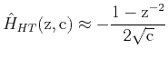
For
=0, the transfer functions of equations A-4
and A-11 are approximated as
 |
(22) |
 |
(23) |
We compare equations A-12 and A-13, and we conclude
that these two transfer functions in middle frequency band of the
frequency domain differ by the constant coefficient
 .
.
|
|
|
|
| Seismic dip estimation based on the two-dimensional Hilbert transform and its application in random noise attenuation | |
|
Next: Bibliography
Up: Appendix A: Hilbert transform
Previous: Derivation of the FIR
2015-05-07