Seismic dip estimation based on the two-dimensional Hilbert transform and its application in random noise attenuation

Noniterative local dip calculation

Following the local plane-wave equation (Fomel, 2002)

$$\frac{\partial{P(x,t})}{\partial{x}}+{\sigma}(x,t) \frac{\partial{P(x,t})}{\partial{t}}=0,$$ (1)

we define the local dip of seismic data

$${\sigma}(x,t)=-\frac{\partial{P(x,t})}{\partial{x}}{\slash} \frac{\partial{P(x,t})}{\partial{t}},$$ (2)

where $P(x,t)$ is the seismic wave field and ${\sigma}(x, t)$ is the local seismic dip as a function of time $t$ and distance $x$ . However, in actual computations, because the local dip is used to determine the direction of a seismic event, we ignore the dimensions and sampling interval; thus, ${\sigma}$ only depends on the sampling data and the local dimensionless dip is defined as

$${\sigma}=-(\frac{\partial{P(x,t})}{\partial{x}}{\slash} \frac{\pa... ...ta}t}= -\frac{\partial{P}}{\partial{x}}{\slash}\frac{\partial{P}}{\partial{y}},$$ (3)

where $\partial{P}{\slash}\partial{x}$ and $\partial{P}{\slash}\partial{y}$ are the partial derivatives of the seismic wave field in the $x-$ and $y-$ direction, respectively, and ${\Delta}x$ and ${\Delta}t$ are the respective sampling intervals in the $x-$ and $y-$ direction.

Using equation 3, we compute the local dip by using the specific values of the space- and time-directional derivatives. Hence, we first discuss the derivative operator.

The ideal differentiator frequency response is

$$F_{IDD}({\omega})=i{\omega},-{\pi}\leq\omega\leq\pi.$$ (4)

The ideal differentiator frequency response is multiplied by a frequency-dependent linear function in the frequency domain. The direct calculation of the derivative of the signal in the time domain enhances the high-frequency random noise and reduces the dip accuracy. Thus, we analyze the frequency response of the derivative operator and the frequency response of the Hilbert transform. We derive the Hilbert transform (Appendix A) and the approximate partial derivative by using the finite impulse response (FIR) filter (Pei and Wang, 2001). We use a 2D Hilbert transform to approximate the partial derivatives of the wave field, which reduces the side effect of strong high-frequency random noise owing to the derivative algorithm.

The redefined noniterative local dip of the seismic data is

$${\sigma} =-(\frac{\partial{P}}{\partial{x}}{\slash} \frac{\partia... ...ac{FFT^{-1} [H_{HT}(x)]}{FFT^{-1}[H_{HT}(y)]}{\approx}-\frac{H_{HTx}}{H_{HTy}},$$ (5)

where $\tilde{P}(x)$ is the frequency response function of the partial derivative in the $x-$ direction and $\tilde{P}(y)$ is the frequency response function of the partial derivative in the $y-$ direction. The dimensions are ignored in the derivation and $c$ does not depend on the time and space sampling intervals; thus, we take $c_x=c_y$ . $H_{HT}(x)$ is the frequency response function of the Hilbert transform in the $x-$ direction and $H_{HT}(y)$ is the frequency response function of the Hilbert transform in the $y-$ direction. $H_{HTx}$ and $H_{HTy}$ are the components of the 2D Hilbert transform in the $x-$ and $y-$ direction, respectively. Using equation 5, we calculate the local seismic dip attribute by using the 2D Hilbert transform instead of the derivative operation. Because division is required in equation 5 and the denominator might become zero, we add the nonzero constant $\varepsilon$ in the denominator

$$\sigma{\approx}-\frac{H_{HTx}}{H_{HTy}+\varepsilon}.$$ (6)

Fomel (2007) proposed the shaping regularization for imposing regularization constraints in estimation problems and defined the local seismic attributes. In this paper, we use the same method to constrain the division and smooth the local dip by using the Gaussian smooth operator as the regularization operator.

noise,nrt,nrx,rizdip
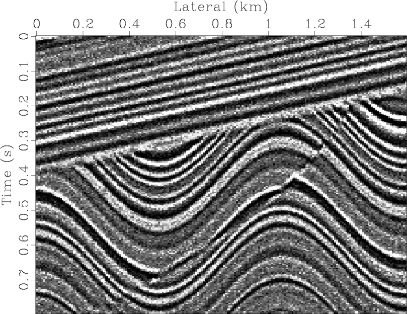
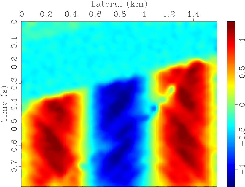
Figure 1. Local seismic dip based on the 2D Hilbert transform. Synthetic seismic data (a), time component of the 2D Hilbert transform (b), space component of the 2D Hilbert transform (c), and local seismic dip (d).

To show the validity of the proposed dip calculation method, we construct a synthetic seismic model and add white Gaussian random noise, as shown in Figure 1a. The components of the 2D Hilbert transform in the $x-$ and $y-$ direction are shown in Figures 1b and 1c, respectively. We obtain the dip of the seismic data by using the ratio of the two components and calculate the smoothing constraints, as shown in Figure 1d. We see that the calculation results can accurately reflect the dip value of the original data at different locations, such as the tilted layers at the top the underlying strata with the sinusoidal fluctuations, and the fault location. Using the 2D Hilbert transform and shaping regularization, we obtain the smooth local dip attribute.

Another effective calculation method of the time-varying and space-variant seismic local dip is based on the plan-wave destruction (PWD) filter proposed by Fomel (2002). The PWD filter realizes the plane-wave propagation across different traces, while the total energy of the propagating wave stays invariant, by using an all-pass digital filter in the time domain and a Taylor expansion of the all-pass filter frequency. We obtain the relation of the PWD and space-time-varying local seismic dip by using the Gauss-Newton algorithm to solve the nonlinear problem of local seismic dip. This method can be essentially understood as solving an implicit finite-difference scheme for the local planewave equation. The disadvantage of the PWD-based calculation method is its slow computation speed, which is especially worse at higher order conditions. The computational cost of the proposed method is proportional to $2N_{x}\times N_{t}$ , where $N_{x}\times N_{t}$ is the data size, whereas the computational efficiency of the PWD-based dip estimation method is proportional to $N_{iter}\times N_{x} \times N_{t}$ , where $N_{iter}$ is the number of iterations. Hence, to achieve similar accuracy, the dip estimation method based on the 2D Hilbert transform requires a smaller number of iterations than the PWD-based method.

The dip of seismic events controls the trend of the constructed seismic model; thus, next, we need to apply filtering along the trend. The selected filtering method must simultaneously suppress the seismic noise and protect structural information.

Seismic dip estimation based on the two-dimensional Hilbert transform and its application in random noise attenuation