|
|
|
|
Seismic data interpolation using generalised velocity-dependent seislet transform |
Next: Discussion Up: Liu et al.: Interpolation Previous: Synthetic Example
|
|
|
|
Seismic data interpolation using generalised velocity-dependent seislet transform |
To evaluate the performance of the proposed method in field
conditions, we used a historic marine dataset from the Gulf of
Mexico (Claerbout, 2000). Figure 7a shows
the input data, in which near-offset information is completely
missing. We removed 40% of randomly selected traces
(Figure 7b) from the input data
(Figure 7a). The velocity scanning from the
missing data can still generate accurate parameter fields using
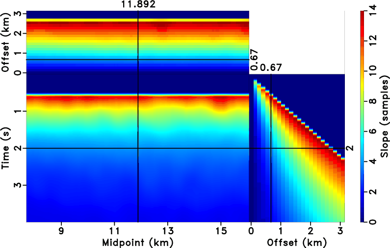
equation 4. Figure 8a and
Figure 8b show the velocity spectra and
![]() spectra, respectively. Equation 5 converts RMS
velocity and
spectra, respectively. Equation 5 converts RMS
velocity and ![]() to seismic pattern
(Figure 8c), which displays the varying
slopes in CMP gathers and common-offset sections. The generalized
velocity-dependent (VD)-seislet transform compresses predictable
information according to the local slopes along the offsets. We
applied the modified Bregman iteration with the generalized
VD-seislet transform to recover missing data. The results show that
the missing traces were interpolated well even when anisotropy is
present (Figure 9b). For comparison, we
applied 3D Fourier transform with POCS
(Figure 9a). The Fourier transform could
not recover the missing information as accurately as the generalized
VD-seislet transform. The results of the 3D Fourier POCS method show
obvious gaps caused by inaccurate interpolation, whereas the
generalized VD-seislet and the modified Bregman iteration strategy
provides a reasonably accurate result for interpolating missing data.
to seismic pattern
(Figure 8c), which displays the varying
slopes in CMP gathers and common-offset sections. The generalized
velocity-dependent (VD)-seislet transform compresses predictable
information according to the local slopes along the offsets. We
applied the modified Bregman iteration with the generalized
VD-seislet transform to recover missing data. The results show that
the missing traces were interpolated well even when anisotropy is
present (Figure 9b). For comparison, we
applied 3D Fourier transform with POCS
(Figure 9a). The Fourier transform could
not recover the missing information as accurately as the generalized
VD-seislet transform. The results of the 3D Fourier POCS method show
obvious gaps caused by inaccurate interpolation, whereas the
generalized VD-seislet and the modified Bregman iteration strategy
provides a reasonably accurate result for interpolating missing data.
If we extend the generalized velocity-dependent (VD)-seislet
transform domain along the transform scale axis and recalculate the
slope field according to the new ![]() -coordinate axis in
equation 5, the inverse generalized VD-seislet transform
will accomplish trace interpolation of the input CMP gather
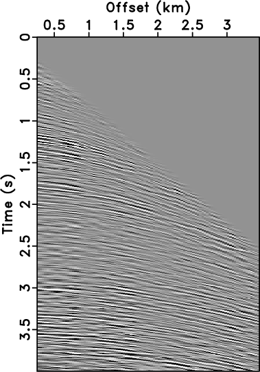
(Figure 10a), which is selected from
Figure 7a at the midpoint location 11.8925
km. We extended the generalized VD-seislet coefficients with small
random noise to consider the existence of realistic noise on
different scale levels. Figure 10b shows that the
interpolated result provides four times more traces and removes most
aliasing. Thus, trace interpolation is a natural operation in the
generalized VD-seislet domain.
-coordinate axis in
equation 5, the inverse generalized VD-seislet transform
will accomplish trace interpolation of the input CMP gather
(Figure 10a), which is selected from
Figure 7a at the midpoint location 11.8925
km. We extended the generalized VD-seislet coefficients with small
random noise to consider the existence of realistic noise on
different scale levels. Figure 10b shows that the
interpolated result provides four times more traces and removes most
aliasing. Thus, trace interpolation is a natural operation in the
generalized VD-seislet domain.


|
|---|
|
bei,bei-zero
Figure 7. Marine data with near-offset missing (a) and data with 40% traces removed (b). |
|
|


|
|---|
|
bei-vel,bei-s,bei-dip
Figure 8. Velocity section (a) and |
|
|


|
|---|
|
bfour3pocs,bei-seis2
Figure 9. Interpolated results using different methods. 3D Fourier POCS method (a) and the proposed method (b). |
|
|

|
|---|
|
cmp1,cmp2
Figure 10. CMP gather before (a) and after (b) trace interpolation. The interpolated gather has four times more traces than the original one shown in Figure 10a. |
|
|
|
|
|
|
Seismic data interpolation using generalised velocity-dependent seislet transform |