|
|
|
|
Seismic data interpolation using streaming prediction filter in the frequency domain |
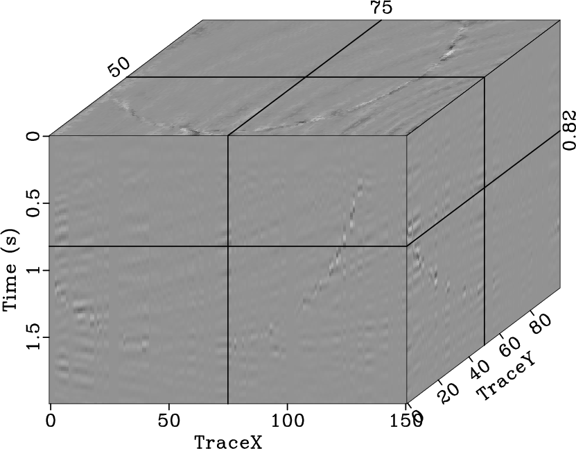
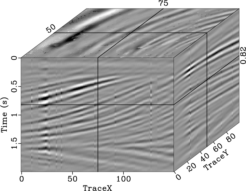
For the 3D data interpolation test, we selected a 3D synthetic model
(Fig. 9a) containing curve events and faults, and the
data cube randomly removed ![]() of the seismic traces, where the
faults were hard to distinguish (Fig. 9c). The
of the seismic traces, where the
faults were hard to distinguish (Fig. 9c). The
![]() -
-![]() -
-![]() spectrum of the synthetic model and the missing
data model are shown in Fig. 9b and 9d,
respectively. Because currently seislet transform can only handle 2D
datasets, here we evaluated the recovery ability of the
spectrum of the synthetic model and the missing
data model are shown in Fig. 9b and 9d,
respectively. Because currently seislet transform can only handle 2D
datasets, here we evaluated the recovery ability of the ![]() -
-![]() -
-![]() SPF by comparing with the 2D seislet POCS method and the 3D Fourier
POCS method. The parameters of the
SPF by comparing with the 2D seislet POCS method and the 3D Fourier
POCS method. The parameters of the ![]() -
-![]() -
-![]() SPF are
SPF are
![]() ,
,
![]() ,
,
![]() , and
11 (space
, and
11 (space ![]() )
) ![]() 6 (space
6 (space ![]() ) filter coefficients. The 2D
seislet POCS does not reconstruct the missing data well
(Fig. 10a), and generates large interpolation errors
(Fig. 10b). The interpolated results
(Fig. 10c and 10e) show that both the 3D
Fourier POCS and the
) filter coefficients. The 2D
seislet POCS does not reconstruct the missing data well
(Fig. 10a), and generates large interpolation errors
(Fig. 10b). The interpolated results
(Fig. 10c and 10e) show that both the 3D
Fourier POCS and the ![]() -
-![]() -
-![]() SPF can recover the missing traces
even when faults are present. However, the interpolation errors
(Fig. 10d and 10f) display that the
SPF can recover the missing traces
even when faults are present. However, the interpolation errors
(Fig. 10d and 10f) display that the
![]() -
-![]() -
-![]() SPF produces less error and preserves the amplitude of the
events reasonably better than the 3D Fourier POCS. The comparison of
the
SPF produces less error and preserves the amplitude of the
events reasonably better than the 3D Fourier POCS. The comparison of
the ![]() -
-![]() -
-![]() spectra is shown in
Fig. 11, the
spectra is shown in
Fig. 11, the ![]() -
-![]() -
-![]() SPF
reduces the influence of aliasing. More importantly, the
SPF
reduces the influence of aliasing. More importantly, the ![]() -
-![]() -
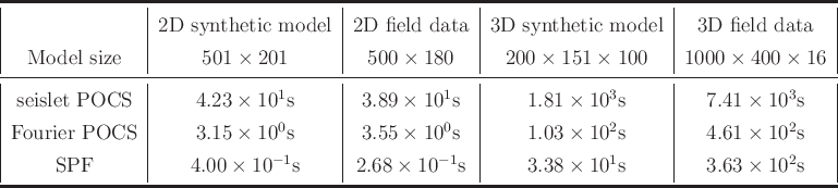
-![]() SPF significantly reduces the computational cost by avoiding the
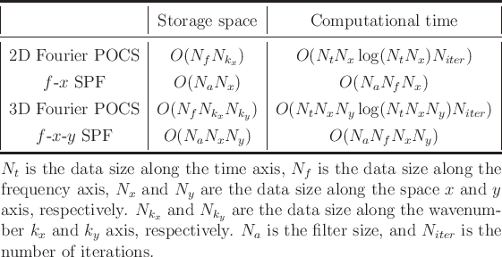
iterative algorithm especially in higher dimensions. Compared with
the Fourier POCS, the proposed methods solve the problem without
iterations, which reduces the computational cost
(Table 1). Table 2 shows the time consumption
of each method, and the computation platform uses 2.0GHz E5-2650 CPU.
SPF significantly reduces the computational cost by avoiding the
iterative algorithm especially in higher dimensions. Compared with
the Fourier POCS, the proposed methods solve the problem without
iterations, which reduces the computational cost
(Table 1). Table 2 shows the time consumption
of each method, and the computation platform uses 2.0GHz E5-2650 CPU.
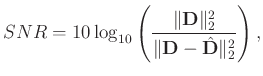
To further evaluate the interpolation ability of the proposed methods, we defined the signal-to-noise ratio (SNR) as a measurement:


|
|---|
|
qdome,fkqd,gapqd,fkgapqd
Figure 9. Synthetic 3D model (a) and |
|
|


|
|---|
|
stpocsqd,errstpocsqd,pocsqd,errpocsqd,spfqd,errspfqd
Figure 10. Reconstructed result (a) and interpolation error (b) using the 2D seislet POCS, reconstructed result (c) and interpolation error (d) using the 3D Fourier POCS, reconstructed result (e) and interpolation error (f) using the 3D |
|
|


|
|---|
|
fkstpocsqd,fkpocsqd,fkspfqd
Figure 11. |
|
|


|
|---|
|
gap3d-5,intp3d-5,gap3d-95,intp3d-95
Figure 12. Model with |
|
|

|
|---|
|
snr3d
Figure 13. The SNR changing with different degree of trace missing (range from |
|
|
We used 3D field common mid-point (CMP) gathers after normal moveout
(NMO) to further test the proposed method (Fig. 14a).
Fig. 14b shows data binning, where the blank space denotes
approximately ![]() of the missing traces. A large amount of missing
traces lead to the spatial aliasing artifacts as shown in
Fig. 18a. The 2D seislet POCS works well with the
horizontal events, but the data interpolation result is not reasonable
where curve and horizontal events intersect
(Fig. 15a). The 3D Fourier POCS can recover most
horizontal events, however, some large gaps remain in
Fig. 16a. We chose
of the missing traces. A large amount of missing
traces lead to the spatial aliasing artifacts as shown in
Fig. 18a. The 2D seislet POCS works well with the
horizontal events, but the data interpolation result is not reasonable
where curve and horizontal events intersect
(Fig. 15a). The 3D Fourier POCS can recover most
horizontal events, however, some large gaps remain in
Fig. 16a. We chose
![]() ,
,
![]() ,
,
![]() , and 101 (space
, and 101 (space ![]() )
) ![]() 5 (space
5 (space ![]() ) filter
coefficients for the
) filter
coefficients for the ![]() -
-![]() -
-![]() SPF. The design of the filter
coefficients is large, which increases the computational
time-consumption of the
SPF. The design of the filter
coefficients is large, which increases the computational
time-consumption of the ![]() -
-![]() -
-![]() SPF. The interpolation result
using the 3D
SPF. The interpolation result
using the 3D ![]() -
-![]() -
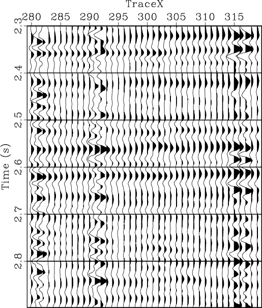
-![]() SPF (Fig. 17a) shows that the
missing traces are reasonably reconstructed, the broken events are
well recovered, and the continuity of both linear and curve events are
interpolated well. A close-up comparison at TraceY=8
(Fig. 15b, 16b, and 17b)
shows that the
SPF (Fig. 17a) shows that the
missing traces are reasonably reconstructed, the broken events are
well recovered, and the continuity of both linear and curve events are
interpolated well. A close-up comparison at TraceY=8
(Fig. 15b, 16b, and 17b)
shows that the ![]() -
-![]() -
-![]() SPF can handle more gaps and recover the
amplitude of nonstationary events better than the 2D seislet POCS and
the 3D Fourier POCS. The
SPF can handle more gaps and recover the
amplitude of nonstationary events better than the 2D seislet POCS and
the 3D Fourier POCS. The ![]() -
-![]() -
-![]() spectra
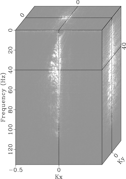
(Fig. 18) demonstrate
that the
spectra
(Fig. 18) demonstrate
that the ![]() -
-![]() -
-![]() SPF can handle aliasing, and the energy is
converged in the
SPF can handle aliasing, and the energy is
converged in the ![]() -
-![]() -
-![]() spectrum
(Fig. 18d).
spectrum
(Fig. 18d).
3.5pt
|


|
|---|
|
gapcmp,mask
Figure 14. 3D field data with trace missing (a) and data binning of the field data (b). |
|
|


|
|---|
|
stpocscmp,stpocszoom
Figure 15. Reconstructed result using the 2D seislet POCS (a), and close-up of the interpolated result (b). |
|
|

|
|---|
|
pocscmp,pocszoom
Figure 16. Reconstructed result using the 3D Fourier POCS (a), and close-up of the interpolated result (b). |
|
|


|
|---|
|
spfcmp,spfzoom
Figure 17. Reconstructed result using the 3D |
|
|


|
|---|
|
fkgapcmp,fkstpocscmp,fkpocscmp,fkspfcmp
Figure 18. The |
|
|
|
|
|
|
Seismic data interpolation using streaming prediction filter in the frequency domain |