|
|
|
|
Nonstationary pattern-based signal-noise separation using adaptive prediction-error filter |
To estimate the nonstationary pattern of a 2D seismic section ![]() ,
prediction coefficients An of the APEF can be obtained as:
,
prediction coefficients An of the APEF can be obtained as:
To obtain the whitening output, one needs to design APEF
![]() of data
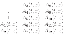
with the causal filter structure. For example, a five-sample (time)
of data
with the causal filter structure. For example, a five-sample (time) ![]() three-sample (space) template is shown as:
three-sample (space) template is shown as:
(i) Random noise: it supposes that the energy of random noise is spatially
uncorrelated, and its statistical property may slightly change with time.
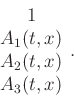
To characterize the model of random noise, noise pattern N can be set as the
shape of a column. The following is an example of the noise pattern structure
with 4 (time) ![]() 1 (space) coefficients:
1 (space) coefficients:
We can generate a noise model containing the characteristics of noise
![]() ,
and calculate APEF
,
and calculate APEF
![]() from the noise model. Also, one can directly
estimate APEF
from the noise model. Also, one can directly
estimate APEF
![]() of random noise from dataset
of random noise from dataset
![]() , especially
when there exists strong random noise in the dataset.
, especially
when there exists strong random noise in the dataset.
![]() with one-column
shape can only capture the temporal spectrum of random noise, but ignores the
signal predictability along the space direction in the dataset.
with one-column
shape can only capture the temporal spectrum of random noise, but ignores the
signal predictability along the space direction in the dataset.
(ii) Ground-roll noise: due to the difference of the dominant frequency, ground-roll
noise and the effective signal can usually be separated in the frequency domain.
Using a low-pass filter to the data can produce a noise model. Similarly, according
to the difference of slowness, the primaries can be muted in the radon domain, and
a ground-roll noise model can be obtained through the inverse radon transform. Here,
we first use a reliable low-pass filter to generate the ground-roll noise model, then
APEF
![]() of the ground-roll noise is calculated according to the structure
similar to that of data as equation 11. Due to the slower speed of
the ground-roll noise, it has steep events with larger local slope, and the filter
size needs to be adjusted to a larger length in the time direction.
of the ground-roll noise is calculated according to the structure
similar to that of data as equation 11. Due to the slower speed of
the ground-roll noise, it has steep events with larger local slope, and the filter
size needs to be adjusted to a larger length in the time direction.
Therefore, the proposed signal-noise separation method exploits a two-step strategy:
(i) estimating data pattern
![]() and noise pattern
and noise pattern
![]() by using
the APEF, and (ii) separating signal and noise with the pattern-based method
(equation 7). The further examination of the proposed method will
be shown in the data examples section.
by using
the APEF, and (ii) separating signal and noise with the pattern-based method
(equation 7). The further examination of the proposed method will
be shown in the data examples section.
|
|
|
|
Nonstationary pattern-based signal-noise separation using adaptive prediction-error filter |
![$\displaystyle \bar{\mathbf{A}}_{n} (t,x) = \arg \min_{A_{n}} \Vert \; \mathbf{d...
...2} \; \sum_{n=1}^{N} \Vert \; \mathbf{R} [\mathbf{A}_{n}(t,x)] \; \Vert _2^2\;,$](img28.png)