|
 |
 |
 | Nonstationary pattern-based signal-noise separation using adaptive prediction-error filter |  |
![[pdf]](icons/pdf.png) |
Next: Estimation of nonstationary pattern
Up: Theory
Previous: Theory
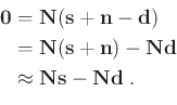
A simple assumption is that the dataset
 can be considered as the
summation of signal
can be considered as the
summation of signal
 and noise
 :
:
 |
(1) |
Usually, signal
represents reflection events or geologic events,
and noise
can be regarded as random noise or ground-roll noise.
Let operators
 and
and
 denote the patterns of signal and
noise, respectively. PEF is reasonable to be the pattern operator as it
approximates the inverse energy spectrum of the corresponding component.
Claerbout (2010) described the pattern operator as the absorbing operator,
for instance, operator
may absorb noise
(
denote the patterns of signal and
noise, respectively. PEF is reasonable to be the pattern operator as it
approximates the inverse energy spectrum of the corresponding component.
Claerbout (2010) described the pattern operator as the absorbing operator,
for instance, operator
may absorb noise
(
 ). And it can destroy the corresponding
noise component from data
and leave signal
:
). And it can destroy the corresponding
noise component from data
and leave signal
:
Meanwhile, operator
absorbs or destroys signal component
:
 |
(3) |
which is used to restrict the shape of signal
. By using above
relationships, the pattern-based method raises a constrained least-squares
problem, and solving such a problem can separate signal
and
noise
from data volume
.
 |
(4) |
where
 is the scaling factor of regularization term, which
balancing the energy between estimated signal
is the scaling factor of regularization term, which
balancing the energy between estimated signal
 and
noise
and
noise
 .
.
In practice, field data d and the noise model are often available, but the
clean signal is not. We here considered the noise model to be a dataset
containing the properties of noise
, and the noise model can
be obtained as a roughly separated noise section. Therefore, data pattern
 and noise pattern
are easily estimated from the field data
and noise model, while it cannot directly obtain signal pattern
.
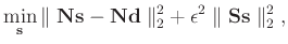
Normally, one makes a compromise by replacing
with
:
with
:
and noise pattern
are easily estimated from the field data
and noise model, while it cannot directly obtain signal pattern
.
Normally, one makes a compromise by replacing
with
:
with
:
 |
(5) |
where
may be unsuitable for constraining the shape of
signal
, and finally lead to undesirable separation result.
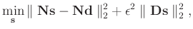
Assuming that noise
and signal
are uncorrelated,
Spitz (1999) proposed an approximation
 ,
which is based on the relationship between the pattern operator and the
energy spectrum of the corresponding component, and the regularization term
becomes
,
which is based on the relationship between the pattern operator and the
energy spectrum of the corresponding component, and the regularization term
becomes
 . Furthermore, one can
multiply equation 5 by
to avoid the acquisition
of
. Furthermore, one can
multiply equation 5 by
to avoid the acquisition
of
 :
:
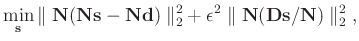 |
(6) |
then the signal-noise separation problem turns into:
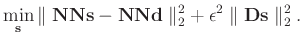 |
(7) |
Equation 7 avoids the requirement for pattern operator
of the clean signal, and minimizing the equation leads to the expression of
the estimated signal:
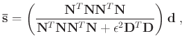 |
(8) |
and the formal solution of the estimated noise is:
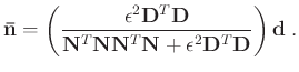 |
(9) |
The conjugate gradient algorithm is implemented to calculate the numerical
solution of equations 8 and 9 (Appendix section).
We will discuss the estimation of the nonstationary pattern operators in
the next section.
|
|
|
|
| Nonstationary pattern-based signal-noise separation using adaptive prediction-error filter | |
|
Next: Estimation of nonstationary pattern
Up: Theory
Previous: Theory
2022-04-11