Shortest path ray tracing on parallel GPU devices

Results and discussion

It is performed a test to compare the velocities of GPU parallel and CPU sequential shortest path ray tracing algorithms with different model sizes and different neighborhood radii. The sequential and parallel versions were executed in an intel icore^TM i7 CPU equipped with a nvidia geforce gt 650m GPU. Although it is not a high-end GPU device it can be useful to show the performance of the parallel ray tracer and better performance is expected from more advanced GPUs. This GPU has the following relevant specifications:

Global memory

$2048$ MBytes.

Computing cores

$384$.

Memory bus width

$128$ bytes.

Shared memory per block

$49152$ bytes.

Threads per block

$1024$.

There were built $16$ velocity models with dimensions ranging from $128\times 128$ vertices to $1600\times 1600$ vertices to test the GPU parallel program performance. All models were a simple vertical gradient with $0.5km/s$ on the top and $4km/s$ on the bottom.

The GPU function kernels were made for a block size of $16\times 16$ threads to meet the maximum number of threads per block and the maximum shared memory per block. The measured times account for all GPU operations: data transfers to and from device, weight precalculation and ray tracing.

The sequential version of the shortest path ray tracer was also tested using the same set of velocity models to provide a point of comparison. This sequential version was implemented with the standard library priority queue that provides a fast implementation of this data structure that dominates the velocity of this algorithm. Both ray tracers, sequential and parallel, were compiled with -O4 optimization flag.

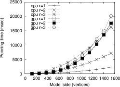
In Figure 7 are shown the time results for three neighborhood radii: $1,2$ and $3$. The CPU version outperforms the parallel one in the first two radii and is almost as good in the third. The reason is that in calculations with low radius values there are not enough operations to keep the GPU busy while waiting for data transfers from global to shared memory.

result1
Figure 7. CPU vs. GPU for three neighborhood radius: $1,2$ and $3$.

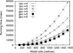
Figure 8 displays the time results for other three neighborhood radii: $4,5$ and $6$. In these cases, the parallel implementation is faster than the sequential one, with a speedup factor between $2$ and $3$ for the highest radius. In these cases the high number of operations per thread was enough to hide the latency of global memory. Despite the low capacity of the GPU device used in the test, this is a significant improvement over the sequential solution. More powerful GPU devices can deliver better improvements.

One important thing to consider involves the memory requirements. The most expensive piece of data is the weight array that has $((2r+1)^2-1)/2$ elements for each model vertex. This imposes a very serious restriction to the model size because of the limited amount of memory in the GPU device. This can be amelioriated with a swapping scheme that loads this array by fragments or by using various GPU devices at the same time. Both possibilities need further experimentation. The possibility of calculating this array on the fly at each iteration is out of the question because it is very time consuming. On the other side, the weight precalculation can be better amortized if varius ray tracings with different sources are going to be performed on the same velocity model, so only one precalculation is needed for all of them.

result2
Figure 8. CPU vs. GPU for three neighborhood radius: $4,5$ and $6$.

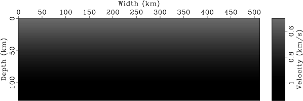
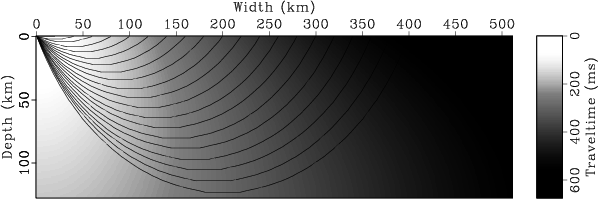
A mild vertical gradient velocity model is shown in Figure 9. The velocity of this model varies with depth $z$: $0.5+0.005z$ in $km/s$. Figure 10 shows a composite image of traveltimes to all model positions and some selected rays using the GPU raytracer with size neighbor equal six, in just one run.

grad
Figure 9. Vertical velocity gradient: $0.5+0.005z$ in $km/s$.

timesrays
Figure 10. Traveltimes to all velocity model positions and some selected rays. Source is at $(0,0)$ position.

Shortest path ray tracing on parallel GPU devices