|
|
|
|
Homework 5 |
|
dune
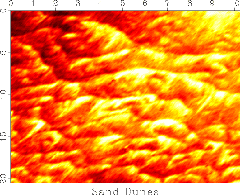
Figure 5. Image of sand dunes in a river. |
|
|---|---|
|
|
Figure 5 shows an image of sand dunes at the bottom of a
river![]() . In this part of the assignment, you
will try to compress the image by applying different transforms.
. In this part of the assignment, you
will try to compress the image by applying different transforms.
|
|---|
|
cos,sort
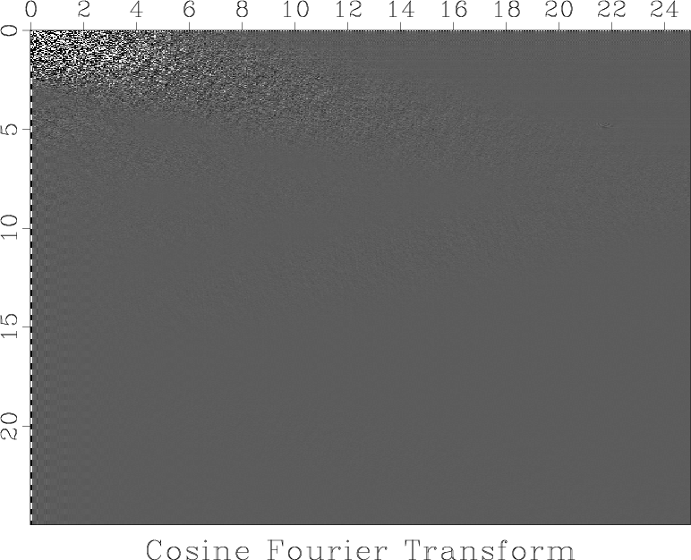
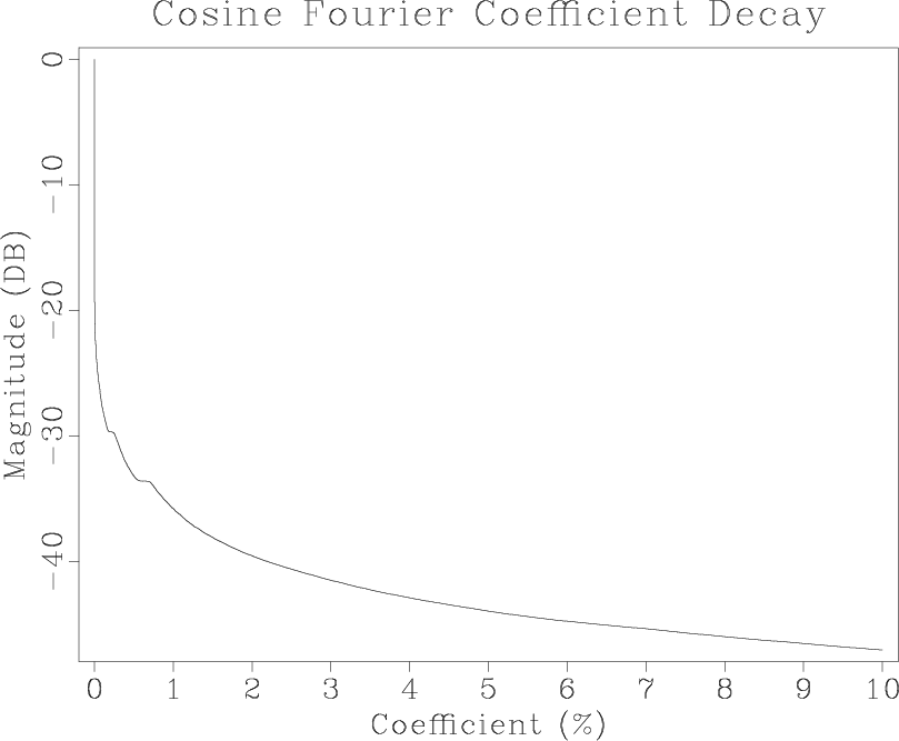
Figure 6. (a) Sand dunes image in the cosine Fourier domain. (b) Fourier coefficients sorted by absolute value and displayed on the logarithmic (decibel) scale. |
|
|
Figure 6a shows the image after applying the cosine transform (a version of the Fourier transform that keeps coefficients real). Notice both compactness and sparsity in the Fourier domain. To analyze the sparsity pattern, Figure 6b shows Fourier coefficients after sorting them by absolute value. The rate of coefficient decay is a measure of sparsity.
|
|---|
|
inv
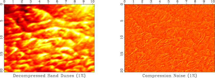
Figure 7. (a) Sand dunes image reconstructed after thresholding. (b) Compression noise. |
|
|
Figure 7 shows the result of shrinkage (soft thresholding) of Fourier coefficients using 1% threshold and the difference between the reconstructed image and the true image.
Your task:
scons viewto reproduce the figures on your screen.
from rsf.proj import *

# Critical parameter
perc = 1 # percentage for thresholding

# Download data
Fetch('dunes3.HH','dunes')
Flow('dunes','dunes3.HH','dd form=native')

# Window size
n1=1024
n2=512

# Plotting macro
def plot(title):
    return '''
    grey color=H bias=-213 clip=150 title="%s"
    ''' % title

# Display data
Flow('dune','dunes','window n3=1 n1=%d n2=%d' % (n1,n2))
Result('dune',plot('Sand Dunes'))

# Transform dictionary
######################
transforms = {
    'cos': ('Cosine Fourier',
            'cosft sign1=1 sign2=1',
            'cosft sign1=-1 sign2=-1'),
    'dwt': ('Digital Wavelet',
            '''
            dwt type=b inv=y unit=y | transp |
            dwt type=b inv=y unit=y | transp
            ''',
            '''
            transp | dwt type=b inv=y unit=y adj=y |
            transp | dwt type=b inv=y unit=y adj=y
            ''')
    }

transform = transforms['cos']

# Apply forward transform
Flow('cos','dune',transform[1])
Result('cos',
       'grey title="%s Transform" ' % transform[0])

# Sort coefficients
Flow('sort','cos',
     '''
     put n1=%d n2=1 d1=%g label1=Coefficient unit1=%% |
     math output="abs(input)" | sort | scale axis=1 |
     math output="10*log(input)/log(10)"
     ''' % (n1*n2,100.0/(n1*n2-1)))
Result('sort',
       '''
       window max1=10 |
       graph title="%s Coefficient Decay"
       label2=Magnitude unit2=DB
       ''' % transform[0])

# Threshold and inverse transform
Flow('thr','cos','threshold pclip=%g' % perc)
Flow('inv','thr',transform[2])
Plot('inv',plot('Decompressed Sand Dunes (%g%%)' % perc))

# Noise = Data - Signal
Flow('diff','dune inv','add scale=1,-1 ${SOURCES[1]}')
Plot('diff',
     plot('Compression Noise (%g%%)' % perc) + ' bias=0')

Result('inv','inv diff','SideBySideIso')

End()
|
|
|
|
|
Homework 5 |