Homework 1

Time-power amplitude-gain correction

Raw seismic reflection data come in the form of shot gathers $S(x,t)$, where $x$ is the offset (horizontal distance from the receiver to the source) and $t$ is recording time. Raw data are inconvenient for analysis because of rapid amplitude decay of seismic waves. The decay can be compensated by multiplying the data by a gain function. A commonly used function is a power of time. The gain-compensated gather is

$$S_\alpha(x,t) = t^{\alpha} S(x,t)\;.$$ (4)

The advantage of the time-power gain is its simplicity and the ability to reverse it by multiplying the data by $t^{-\alpha}$. What value of $\alpha$ should one use? Claerbout (1985) argues in favor of $\alpha=2$: one factor of $t$ comes from geometrical spreading and the other from scattering attenuation. Your task is to develop an algorithm for finding a better value of $\alpha$ for a given dataset.

tpow
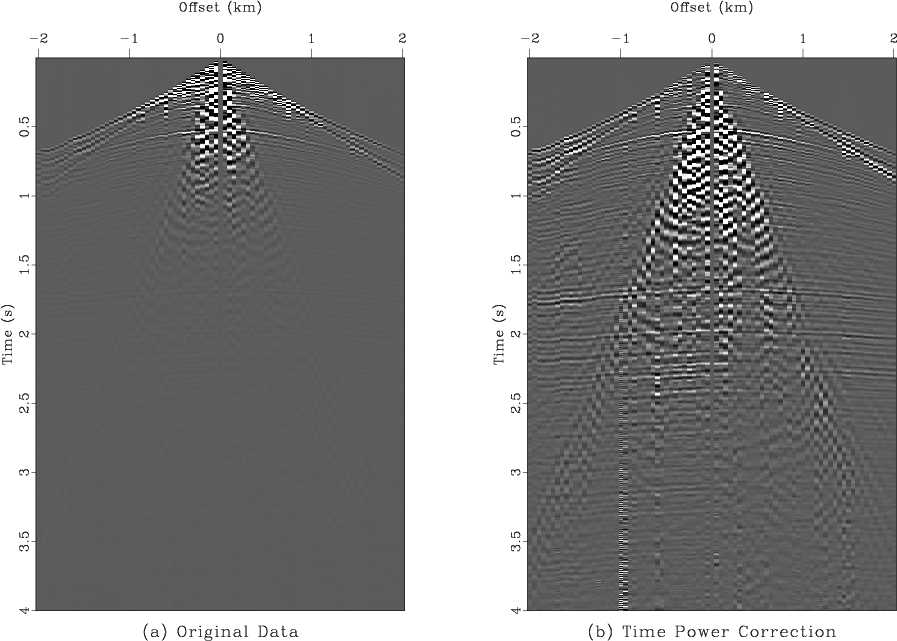
Figure 3. Seismic shot record before and after time-power gain correction.

Figure 3 shows a seismic shot record before and after applying the time-power gain (4) with $\alpha=2$. Start by reproducing this figure on your screen.

1. Change directory to hw1/tpow
2. Run

   scons tpow.view
   

3. Edit the SConstruct file. Find where the value of $\alpha$ is specified in this file and try changing it to a different value. Run scons tpow.view again to check the result.
4. How can we detect if the distribution of amplitudes after the gain correction is uniform? Suggest a measure (an objective function) that would take $S_\alpha(x,t)$ and produce one number that measures uniformity.
5. By modifying the program objective.c, compute your objective function for different values of $\alpha$ and display it in a figure. Does the function appear to have a unique minimum or maximum?

   #include <rsf.h>
   
   int main(int argc, char* argv[])
   {
       int it, nt, ix, nx, ia, na;
       float *trace, *ofunc;
       float a, a0, da, t, t0, dt, s;
       sf_file in, out;
   
       /* initialization */
       sf_init(argc,argv);
       in = sf_input("in");
       out = sf_output("out");
   
       /* get trace parameters */
       if (!sf_histint(in,"n1",&nt)) sf_error("Need n1=");
       if (!sf_histfloat(in,"d1",&dt)) dt=1.;
       if (!sf_histfloat(in,"o1",&t0)) t0=0.;
   
       /* get number of traces */
       nx = sf_leftsize(in,1);
   
       if (!sf_getint("na",&na)) na=1;
       /* number of alpha values */
       if (!sf_getfloat("da",&da)) da=0.;
       /* increment in alpha */
       if (!sf_getfloat("a0",&a0)) a0=0.;
       /* first value of alpha */
   
       /* change output data dimensions */
       sf_putint(out,"n1",na);
       sf_putint(out,"n2",1);
       sf_putfloat(out,"d1",da);
       sf_putfloat(out,"o1",a0);
   
       trace = sf_floatalloc(nt);
       ofunc = sf_floatalloc(na);
   
       /* initialize */
       for (ia=0; ia < na; ia++) {
   	ofunc[ia] = 0.;
       }
   
       /* loop over traces */
       for (ix=0; ix < nx; ix++) {
   
   	/* read data */
   	sf_floatread(trace,nt,in);
   
   	/* loop over alpha */
   	for (ia=0; ia < na; ia++) {
   	    a = a0+ia*da;
   
   	    /* loop over time samples */
   	    for (it=0; it < nt; it++) {
   		t = t0+it*dt;
   
   		/* apply gain t^alpha */
   		s = trace[it]*powf(t,a);
   		
                   /* !!! MODIFY THE NEXT LINE !!! */
   		ofunc[ia] += s*s; 
   	    }
   	}
       }
   
       /* write output */
       sf_floatwrite(ofunc,na,out);
   
       exit(0);
   }
   

6. Suggest an algorithm for finding an optimal value of $\alpha$ by minimizing or maximizing the objective function. Your algorithm should be able to find the optimal value without scanning all possible values. Hint: if the objective function is $f(\alpha)=F[S_\alpha(x,t)]$ and
   

   $$f(\alpha) \approx f(\alpha_0) + f'(\alpha_0) (\alpha-\alpha_0) + \frac{f''(\alpha_0)}{2} (\alpha-\alpha_0)^2$$ (5)

   
   
   then what is the optimal $\alpha$?
7. EXTRA CREDIT for implementing your algorithm for an automatic estimation of $\alpha$ and testing it on the shot gather from Figure 3.

from rsf.proj import *

# Download data 
Fetch('wz.25.H','wz')

# Convert and window
Flow('data','wz.25.H',
     '''
     dd form=native | window min2=-2 max2=2 | 
     put label1=Time label2=Offset unit1=s unit2=km
     ''')

# Display
Plot('data','grey title="(a) Original Data"')
Plot('tpow','data',
     'pow pow1=2 | grey title="(b) Time Power Correction" ')

Result('tpow','data tpow','SideBySideAniso')

# Compute objective function
prog = Program('objective.c')
Flow('ofunc','data %s' % prog[0],
     './${SOURCES[1]} na=21 da=0.1 a0=1')

Result('ofunc',
       '''
       scale axis=1 | 
       graph title="Objective Function" 
       label1=alpha label2= unit1= unit2=
       ''')

End()

Homework 1