|
|
|
|
Homework 1 |
|
byte
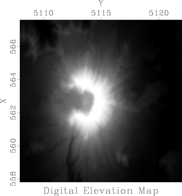
Figure 1. Digital elevation map of Mount St. Helens area. |
|
|---|---|
|
|
Figure 1 shows a digital elevation map of the Mount St. Helens area in Washington. Start by reproducing this figure on your screen.
hw1/dem
scons byte.view
sfin byte.rsfto check the data size and format.
sfattr < byte.rsfto check data attributes. What is the maximum and minimum value? What is the mean value? For an explanation of different attributes, run sfattr without input.
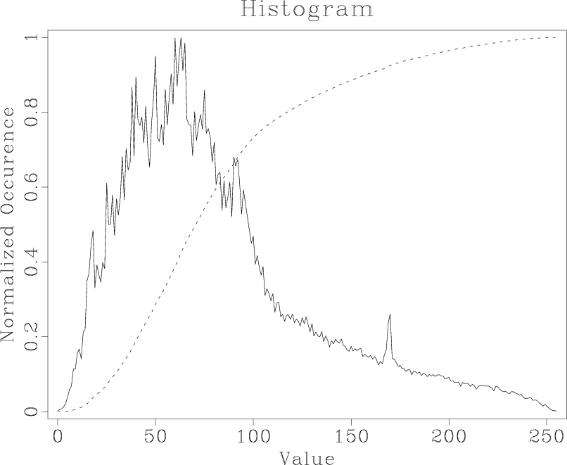
Each image has a certain distribution of values (a histogram). The histogram for the elevation map values is shown in Figure 2. When different values in a histogram are not uniformly distributed, the image can have a low contrast. One way of improving the contrast is histogram equalization.
|
hist
Figure 2. Normalized histogram (solid line) and cumulative histogram (dashed line) of the digital elevation data. |
|
|---|---|
|
|
Let ![]() be the original image. The equalized image will be
be the original image. The equalized image will be
![]() . Let
. Let ![]() be the histogram (probability distribution) of
the original image values. Let
be the histogram (probability distribution) of
the original image values. Let ![]() be the histogram of the modified
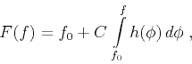
image. The mapping of probabilities suggests
be the histogram of the modified
image. The mapping of probabilities suggests
The algorithm for histogram equalization consists of the following three steps:
Your task:
scons hist.viewto display the figure on your screen.
from rsf.proj import *

# Download data
txt = 'st-helens_after.txt'
Fetch(txt,'data',
      server='https://raw.githubusercontent.com',
      top='agile-geoscience/notebooks/master')
Flow('data.asc',txt,'/usr/bin/tail -n +6')

# Convert to RSF format
Flow('data','data.asc',
     '''
     echo in=$SOURCE data_format=ascii_float
     label=Elevation unit=m
     n1=979  o1=557.805  d1=0.010030675 label1=X
     n2=1400 o2=5107.965 d2=0.010035740 label2=Y |
     dd form=native |
     clip2 lower=0 | lapfill grad=y niter=200
     ''')

# Convert to byte form
Flow('byte','data',
     '''
     dd form=native |
     byte pclip=100 allpos=y bias=2231
     ''')

# Display
Result('byte',
       '''
       grey yreverse=n screenratio=1
       title="Digital Elevation Map"
       ''')

# Histogram
Flow('hist','byte',
     '''
     dd type=float |
     histogram n1=256 o1=0 d1=1 |
     dd type=float
     ''')
Plot('hist',
     'graph label1=Value label2=Occurence title=Histogram')

# Cumulative histogram
Flow('cumu','hist','causint')

Result('hist','hist cumu',
       '''
       cat axis=2 ${SOURCES[1]} | scale axis=1 |
       graph label1=Value label2="Normalized Occurence"
       title=Histogram dash=0,1
       ''')

# ADD HISTOGRAM EQUALIZATION

End()
|
|
|
|
|
Homework 1 |