|
|
|
|
Homework 5 |
Your task: Design an approximation that would be more accurate
than approximation (2). Your approximation should be
suitable for a digital filter implementation in the space
domain. Therefore, it can involve ![]() only through
only through
![]() functions with integer
functions with integer ![]() .
.
cd hw5/hyper
scons viewto generate figures and display them on your screen.
scons viewagain to observe the differences.

|
|---|
|
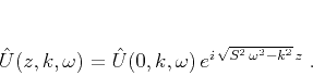
model
Figure 1. Synthetic velocity model with a hyperbolic reflector. |
|
|

|
|---|
|
shot
Figure 2. Synthetic shot gather. Left: Modeled for receivers at the surface. Middle: Receivers extrapolated to 1 km in depth with an exact phase-shift extrapolation operator. Right: Receivers extrapolated to 1 km in depth with an approximate extrapolation operator. |
|
|
|
phase
Figure 3. Phase of the extrapolation operator at 5 Hz frequency as a function of the wave propagation angle. Solid line: exact extrapolator. Dashed line: approximate extrapolator. |

|
|---|---|
|
|
from rsf.proj import *
from math import pi

# Make a reflector model
Flow('refl',None,
     '''
     math n1=10001 o1=-4 d1=0.001 output="sqrt(1+x1*x1)"
     ''')
Flow('model','refl',
     '''
     unif2 n1=201 d1=0.01 v00=1,2 |
     put label1=Depth unit1=km label2=Lateral unit2=km
     label=Velocity unit=km/s |
     smooth rect1=3
     ''')
Result('model',
       '''
       window min2=-1 max2=2 j2=10 |
       grey allpos=y title=Model
       scalebar=y barreverse=y
       ''')

# Reflector dip
Flow('dip','refl','math output="x1/input" ')

# Kirchoff modeling
Flow('shot','refl dip',
     '''
     kirmod nt=1501 twod=y vel=1 freq=10
     ns=1 s0=1 ds=0.01 nh=801 dh=0.01 h0=-4
     dip=${SOURCES[1]} verb=y |
     costaper nw2=200
     ''')
Plot('shot',
     '''
     window min2=-2 max2=2 min1=1 max1=4 |
     grey title="0 km Depth"
     label1=Time unit1=s label2=Offset unit2=km
     labelsz=10 titlesz=15 grid=y
     ''')

# Double Fourier transform

Flow('kw','shot','fft1 | fft3 axis=2')

# Extrapolation filters

dx = 0.01
dz = 1

dx2 = 2*pi*dx
dz2 = 2*pi*dz
a = 0.5*dz2/(dx2*dx2)

# In the expressions below,
# x1 refers to omega and x2 refers to k

Flow('exact','kw',
     'math output="exp(I*sqrt(x1*x1-x2*x2)*%g)" ' % dz2)

Flow('approximate','kw',
     '''
     window f1=1 |
     math output="exp(I*x1*%g)*
     (x1+I*(cos(x2*%g)-1)*%g)/
     (x1-I*(cos(x2*%g)-1)*%g)" |
     pad beg1=1
     ''' % (dz2,dx2,a,dx2,a))

# Extrapolation

for case in ('exact','approximate'):
    Flow('phase-'+case,case,
         '''
         window n1=1 min1=5 min2=-2 max2=2 |
         math output="log(input)" | sfimag
         ''')
    Flow('angle-'+case,'phase-'+case,
         '''
         math output="%g*asin(x1/5)" |
         cmplx $SOURCE
         ''' % (180/pi))

    Flow('shot-'+case,['kw',case],
         '''
         mul ${SOURCES[1]} |
         fft3 axis=2 inv=y | fft1 inv=y
         ''')
    Plot('shot-'+case,
         '''
         window min2=-2 max2=2 min1=1 max1=4 |
         grey title="%g km Depth (%s)"
         label1=Time unit1=s label2=Offset unit2=km
         labelsz=10 titlesz=15 grid=y
         ''' % (dz, case.capitalize()))

Result('shot','shot shot-exact shot-approximate',
       'SideBySideAniso')

Result('phase','angle-exact angle-approximate',
       '''
       cat axis=2 ${SOURCES[1]} |
       graph title=Phase dash=0,1
       label1="Angle From Vertical" unit1="ô_"
       ''')

End()
|
Your task: Change the program for reverse-time migration to implement forward-time modeling using the ``exploding reflector'' approach.
cd hw6/hyper2
scons viewto generate figures and display them on your screen.
scons wave.vplto observe a movie of reverse-time wave extrapolation.
scons viewagain to observe the differences.


|
|---|
|
data,image
Figure 4. (a) Synthetic zero-offset data corresponding to the model in Figure 1. (b) Image generated by reverse-time exploding-reflector migration. The location of the exact reflector is indicated by a curve. |
|
|
from rsf.proj import *

# Make a reflector model
Flow('refl',None,
     '''
     math n1=10001 o1=-4 d1=0.001 output="sqrt(1+x1*x1)"
     ''')
Flow('model','refl',
     '''
     window min1=-3 max1=3 j1=5  |
     unif2 n1=401 d1=0.005 v00=1,2 |
     put label1=Depth unit1=km label2=Lateral unit2=km |
     smooth rect1=3
     ''')

Plot('model',
     '''
     window min2=-1 max2=2 |
     grey allpos=y bias=1 title=Model
     ''')
Plot('refl',
     '''
     graph wanttitle=n wantaxis=n yreverse=y
     min1=-1 max1=2 min2=0 max2=2
     plotfat=3 plotcol=4
     ''')
Result('model','model refl','Overlay')

# Kirchoff zero-offset modeling
Flow('dip','refl','math output="x1/input" ')

Flow('data','refl dip',
     '''
     kirmod nt=1501 dt=0.004 freq=10
     ns=1201 s0=-3 ds=0.005 nh=1 dh=0.01 h0=0
     twod=y vel=1 dip=${SOURCES[1]} verb=y |
     window | costaper nw2=200
     ''')
Result('data',
     '''
     window min2=-2 max2=2 min1=1 max1=4 |
     grey title="Zero-Offset Data" grid=y
     label1=Time unit1=s label2=Distance unit2=km
     ''')

# Reverse-time migration
proj = Project()

# To do the coding assignment in Python,
# comment the next line and uncomment the lines below
prog = proj.Program('rtm.c')

#prog = proj.Command('rtm.exe','rtm.py','cp $SOURCE $TARGET')
#AddPostAction(prog,Chmod(prog,0o755))

Flow('image wave','model %s data' % prog[0],
     '''
     pad beg1=200 end1=200 | math output=0.5 |
     ./${SOURCES[1]} data=${SOURCES[2]}
     wave=${TARGETS[1]} jt=20 n0=200
     ''')

# Display wave propagation movie
Plot('wave',
     '''
     window min2=-1 max2=2 min1=0 max1=2 f3=33 |
     grey wanttitle=n gainpanel=all
     ''',view=1)

# Display image
Plot('image',
     '''
     window min2=-1 max2=2 min1=0 max1=2 |
     grey title=Image
     ''')
Result('image','image refl','Overlay')

End()
|
/* 2-D zero-offset reverse-time migration */
#include <rsf.h>

#ifdef _OPENMP
#include <omp.h>
#endif

static int n1, n2;
static float c0, c11, c21, c12, c22;

static void laplacian(float **uin  /* [n2][n1] */,
		      float **uout /* [n2][n1] */)
/* Laplacian operator, 4th-order finite-difference */
{
    int i1, i2;

#ifdef _OPENMP
#pragma omp parallel for	                       private(i2,i1)		                       shared(n2,n1,uout,uin,c11,c12,c21,c22,c0)
#endif
    for (i2=2; i2 < n2-2; i2++) {
	for (i1=2; i1 < n1-2; i1++) {
	    uout[i2][i1] =
		c11*(uin[i2][i1-1]+uin[i2][i1+1]) +
		c12*(uin[i2][i1-2]+uin[i2][i1+2]) +
		c21*(uin[i2-1][i1]+uin[i2+1][i1]) +
		c22*(uin[i2-2][i1]+uin[i2+2][i1]) +
		c0*uin[i2][i1];
	}
    }
}

int main(int argc, char* argv[])
{
    int it,i1,i2;        /* index variables */
    int nt,n12,n0,nx, jt;
    float dt,dx,dz, dt2,d1,d2;

    float  **vv, **dd;
    float  **u0,**u1,u2,**ud; /* tmp arrays */

    sf_file data, imag, modl, wave; /* I/O files */

    /* initialize Madagascar */
    sf_init(argc,argv);

    /* initialize OpenMP support */
    omp_init();

    /* setup I/O files */
    modl = sf_input ("in");   /* velocity model */
    imag = sf_output("out");  /* output image */

    data = sf_input ("data"); /* seismic data */
    wave = sf_output("wave"); /* wavefield */

    /* Dimensions */
    if (!sf_histint(modl,"n1",&n1)) sf_error("n1");
    if (!sf_histint(modl,"n2",&n2)) sf_error("n2");

    if (!sf_histfloat(modl,"d1",&dz)) sf_error("d1");
    if (!sf_histfloat(modl,"d2",&dx)) sf_error("d2");

    if (!sf_histint  (data,"n1",&nt)) sf_error("n1");
    if (!sf_histfloat(data,"d1",&dt)) sf_error("d1");

    if (!sf_histint(data,"n2",&nx) || nx != n2)
	sf_error("Need n2=%d in data",n2);

    n12 = n1*n2;

    if (!sf_getint("n0",&n0)) n0=0;
    /* surface */
    if (!sf_getint("jt",&jt)) jt=1;
    /* time interval */

    sf_putint(wave,"n3",1+(nt-1)/jt);
    sf_putfloat(wave,"d3",-jt*dt);
    sf_putfloat(wave,"o3",(nt-1)*dt);

    dt2 = dt*dt;

    /* set Laplacian coefficients */
    d1 = 1.0/(dz*dz);
    d2 = 1.0/(dx*dx);

    c11 = 4.0*d1/3.0;
    c12=  -d1/12.0;
    c21 = 4.0*d2/3.0;
    c22=  -d2/12.0;
    c0  = -2.0 * (c11+c12+c21+c22);

    /* read data and velocity */
    dd = sf_floatalloc2(nt,n2);
    sf_floatread(dd[0],nt*n2,data);

    vv = sf_floatalloc2(n1,n2);
    sf_floatread(vv[0],n12,modl);

    /* allocate temporary arrays */
    u0=sf_floatalloc2(n1,n2);
    u1=sf_floatalloc2(n1,n2);
    ud=sf_floatalloc2(n1,n2);

    for (i2=0; i2<n2; i2++) {
	for (i1=0; i1<n1; i1++) {
	    u0[i2][i1]=0.0;
	    u1[i2][i1]=0.0;
	    ud[i2][i1]=0.0;
	    vv[i2][i1] *= vv[i2][i1]*dt2;
	}
    }

    /* Time loop */
    for (it=nt-1; it >= 0; it-) {
	sf_warning("%d;",it);

	laplacian(u1,ud);

#ifdef _OPENMP
#pragma omp parallel for	         private(i2,i1,u2)		         shared(ud,vv,it,u1,u0,dd,n0)
#endif
	for (i2=0; i2<n2; i2++) {
	    for (i1=0; i1<n1; i1++) {
		/* scale by velocity */
		ud[i2][i1] *= vv[i2][i1];

		/* time step */
		u2 =
		    2*u1[i2][i1]
		    - u0[i2][i1]
		    + ud[i2][i1];

		u0[i2][i1] = u1[i2][i1];
		u1[i2][i1] = u2;
	    }

	    /* inject data */
	    u1[i2][n0] += dd[i2][it];
	}

	if (0 == it%jt)
	    sf_floatwrite(u1[0],n12,wave);
    }
    sf_warning(".");

    /* output image */
    sf_floatwrite(u1[0],n12,imag);

    exit (0);
}
|
#!/usr/bin/env python

import sys
import numpy
import m8r

class Laplacian:
    'Laplacian operator, 4th-order finite-difference'

    def __init__(self,d1,d2):
        self.c11 = 4.0*d1/3.0
        self.c12=  -d1/12.0
        self.c21 = 4.0*d2/3.0
        self.c22=  -d2/12.0
        self.c1  = -2.0*(self.c11+self.c12)
        self.c2  = -2.0*(self.c21+self.c22)

    def apply(self,uin,uout):
        n1,n2 = uin.shape

        uout[2:n1-2,2:n2-2] =           self.c11*(uin[1:n1-3,2:n2-2]+uin[3:n1-1,2:n2-2]) +           self.c12*(uin[0:n1-4,2:n2-2]+uin[4:n1  ,2:n2-2]) +           self.c1*uin[2:n1-2,2:n2-2] +           self.c21*(uin[2:n1-2,1:n2-3]+uin[2:n1-2,3:n2-1]) +           self.c22*(uin[2:n1-2,0:n2-4]+uin[2:n1-2,4:n2  ]) +           self.c2*uin[2:n1-2,2:n2-2]

par = m8r.Par()

# setup I/O files
modl=m8r.Input()       # velocity model
imag=m8r.Output()      # output image

data=m8r.Input ('data') # seismic data
wave=m8r.Output('wave') # wavefield

# Dimensions
n1 = modl.int('n1')
n2 = modl.int('n2')

dz = modl.float('d1')
dx = modl.float('d2')

nt = data.int('n1')
dt = data.float('d1')

nx = data.int('n2')
if nx != n2:
    raise RuntimeError('Need n2=%d in data',n2)

n0 = par.int('n0',0) # surface
jt = par.int('jt',1) # time interval

wave.put('n3',1+(nt-1)/jt)
wave.put('d3',-jt*dt)
wave.put('o3',(nt-1)*dt)

dt2 =    dt*dt

# set Laplacian coefficients
laplace = Laplacian(1.0/(dz*dz),1.0/(dx*dx))

# read data and velocity
dd = numpy.zeros([n2,nt],'f')
data.read(dd)
vv = numpy.zeros([n2,n1],'f')
modl.read(vv)

# allocate temporary arrays
u0 = numpy.zeros([n2,n1],'f')
u1 = numpy.zeros([n2,n1],'f')
ud = numpy.zeros([n2,n1],'f')

vv *= vv*dt2

# Time loop
for it in range(nt-1,-1,-1):
    sys.stderr.write("%d" % it)

    laplace.apply(u1,ud)

    # scale by velocity
    ud *= vv

    # time step
    u2 = 2*u1 - u0 + ud
    u0 = u1
    u1 = u2

    # inject data
    u1[:,n0] += dd[:,it]

    if 0 == it%jt:
        wave.write(u1)

# output image
imag.write(u1)
|


|
|---|
|
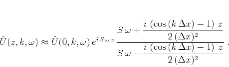
zvel,zref
Figure 5. (a) Sigsbee velocity model. (b) Approximate reflectivity of the Sigsbee model (an ideal image). |
|
|
Your task: Apply your exploding-reflector modeling and migration program from the previous task to generate zero-offset data for Sigsbee and image it.
cd hw6/sigsbee
scons viewto generate figures and display them on your screen.
from rsf.proj import *

# Download velocity model from the data server
##############################################
vstr = 'sigsbee2a_stratigraphy.sgy'
Fetch(vstr,'sigsbee')
Flow('zvstr',vstr,'segyread read=data')

Flow('zvel','zvstr',
     '''
     put d1=0.025 o2=10.025 d2=0.025
     label1=Depth unit1=kft label2=Lateral unit2=kft |
     scale dscale=0.001
     ''')

Result('zvel',
       '''
       window f1=200 |
       grey title=Velocity titlesz=7 color=j
       screenratio=0.3125 screenht=4 labelsz=5
       mean=y
       ''')

# Compute approximate reflectivity
##################################
Flow('zref','zvel',
     '''
     depth2time velocity=$SOURCE nt=2501 dt=0.004 |
     ai2refl | ricker1 frequency=10 |
     time2depth velocity=$SOURCE
     ''')

Result('zref',
       '''
       window f1=200 |
       grey title=Reflectivity titlesz=7
       screenratio=0.3125 screenht=4 labelsz=5
       ''')

End()
|
Figure 6b shows an idealized image (band-passed
reflectivity) for the synthetic model. In ``exploding-reflector''
modeling, this image is assumed to be the seismic wavefield frozen at
zero time. The modeling program extrapolates the wavefield to the
surface and is implemented in phaseshift.c. The program
operates in the frequency-wavenumber domain and establishes a linear
relationship between reflectivity as a function of depth and
zero-offset data as a function of frequency for one space wavenumber.
If we think of this linear relationship as a matrix multiplication, we
can associate forward modeling with multiplication
Figure 7 shows the result of forward modeling
(multiplication by ![]() ) after inverse Fourier transform to
time and space. Your task is to implement the corresponding migration
(multiplication by
) after inverse Fourier transform to
time and space. Your task is to implement the corresponding migration
(multiplication by ![]() ).
).
Instead of simply applying the adjoint operator, we can also try to compute
the least-squares inverse

|
|---|
|
lmodel,expl
Figure 6. (a) Synthetic model: curved reflectors in a |
|
|

|
|---|
|
modl
Figure 7. Zero-offset data generated by exploding-reflector phase-shift modeling. |
|
|
cd hw5/lsmig
scons viewto generate the figures and display them on your screen.
scons migr.view
sfcdottest ./phaseshift.exe mod=kexpl.rsf dat=kmodl.rsf \
vel=vofz.rsf nw=247 dw=0.16276
On a machine with multiple CPUs, you can also try
sfcdottest sfomp ./phaseshift.exe split=2 \
mod=kexpl.rsf dat=kmodl.rsf vel=vofz.rsf nw=247 dw=0.16276
If your adjoint is correct, you should see two identical sets of numbers, such as
sfcdottest:  L[m]*d=(25264,-20273.9)
sfcdottest: L'[d]*m=(25264,-20273.9)
Your actual numbers will be different because of random input vectors but they should be the same between
L[m]*d and L'[d]*m.
scons invs.viewDo you notice any difference with the previous result? Increase the number of iterations from 10 to 100 and repeat the experiment.
from rsf.proj import *

# Generate a reflector model

layers = (
     ((0,2),(3.5,2),(4.5,2.5),(5,2.25),
       (5.5,2),(6.5,2.5),(10,2.5)),
     ((0,2.5),(10,3.5)),
     ((0,3.2),(3.5,3.2),(5,3.7),
       (6.5,4.2),(10,4.2)),
     ((0,4.5),(10,4.5))
)

nlays = len(layers)
for i in range(nlays):
     inp = 'inp%d' % i
     Flow(inp+'.asc',None,
          '''
          echo %s in=$TARGET
          data_format=ascii_float n1=2 n2=%d
          ''' %            (' '.join(map(lambda x: ' '.join(map(str,x)),
                           layers[i])),len(layers[i])))

dim1 = 'o1=0 d1=0.05 n1=201'
Flow('lay1','inp0.asc',
     'dd form=native | spline %s fp=0,0' % dim1)
Flow('lay2',None  ,
     'math %s output="2.5+x1*0.1" '      % dim1)
Flow('lay3','inp2.asc',
     'dd form=native | spline %s fp=0,0' % dim1)
Flow('lay4',None  ,'math %s output=4.5'  % dim1)

Flow('lays','lay1 lay2 lay3 lay4',
     'cat axis=2 ${SOURCES[1:4]}')

graph = '''
graph min1=2.5 max1=7.5 min2=0 max2=5
yreverse=y wantaxis=n wanttitle=n screenratio=1
'''
Plot('lays0','lays',graph + ' plotfat=10 plotcol=0')
Plot('lays1','lays',graph + ' plotfat=2 plotcol=7')
Plot('lays2','lays',graph + ' plotfat=2')

# Velocity

Flow('vofz',None,
     '''
     math output="1.5+0.25*x1"
     d2=0.05 n2=201 d1=0.01 n1=501
     label1=Depth unit1=km
     label2=Distance unit2=km
     label=Velocity unit=km/s
     ''')
Plot('vofz',
     '''
     window min2=2.75 max2=7.25 |
     grey color=j allpos=y bias=1.5
     title=Model screenratio=1
     ''')

Result('lmodel','vofz lays0 lays1','Overlay')

# Exploding reflector

Flow('expl','lays vofz',
     '''
     unif2 d1=0.01 n1=501 v00=1,2,3,4,5 |
     depth2time velocity=${SOURCES[1]} |
     ai2refl | ricker1 frequency=10 |
     time2depth velocity=${SOURCES[1]} |
     put label1=Depth unit1=km
     label2=Distance unit2=km
     ''')

Result('expl',
       '''
       window max1=5 min2=2.5 max2=7.5 |
       grey title="Exploding Reflector" screenratio=1
       ''')

# Modeling
##########

proj = Project()
prog = proj.Program('phaseshift.c')

# Cosine Fourier transform
Flow('kexpl','expl','cosft sign2=1 | rtoc')

Flow('kmodl','kexpl %s vofz' % prog[0],
     '''
     ./${SOURCES[1]} vel=${SOURCES[2]}
     nw=247 dw=0.16276
     ''')

Flow('modl','kmodl',
     'pad n1=769 | fft1 inv=y | cosft sign2=-1')

Result('modl',
       '''
       grey title="Exploding Reflector Modeling"
       label1=Time unit1=s
       ''')

# Migration
###########

Flow('kdata','modl',
     'cosft sign2=1 | fft1 | window n1=247')

Flow('kmigr','kdata %s vofz' % prog[0],
     './${SOURCES[1]} vel=${SOURCES[2]} adj=1')

Flow('migr','kmigr','real | cosft sign2=-1')

# !!! UNCOMMENT BELOW !!!

#Result('migr',
#       '''
#       window max1=5 min2=2.5 max2=7.5 |
#       grey title="Exploding Reflector Migration"
#       screenratio=1 label1=Depth unit1=km
#       ''')

# Least-Squares Migration
#########################

Flow('kinvs','kdata %s vofz kmigr' % prog[0],
     '''
     cconjgrad ./${SOURCES[1]} split=2
     nw=247 dw=0.16276
     vel=${SOURCES[2]} mod=${SOURCES[3]} niter=10
     ''')

Flow('invs','kinvs','real | cosft sign2=-1')

# !!! UNCOMMENT BELOW !!!

#Result('invs',
#       '''
#       window max1=5 min2=2.5 max2=7.5 |
#       grey title="Exploding Reflector LS Migration"
#       screenratio=1 label1=Depth unit1=km
#       ''')


End()
|
/* Phase-shift modeling and migration */

#include <rsf.h>

int main(int argc, char* argv[])
{
    bool adj;
    int ik, iw, nk, nw, iz, nz;
    float k, dk, k0, dw, dz, z0, *v, eps;
    sf_complex *dat, *mod, w2, ps, wave;
    sf_file inp, out, vel;

    sf_init(argc,argv);

    if (!sf_getbool("adj",&adj)) adj=false;
    /* adjoint flag, 0: modeling, 1: migration */

    inp = sf_input("in");
    out = sf_output("out");
    vel = sf_input("vel"); /* velocity file */

    if (!sf_histint(vel,"n1",&nz))
	sf_error("No n1= in vel");
    if (!sf_histfloat(vel,"d1",&dz))
	sf_error("No d1= in vel");
    if (!sf_histfloat(vel,"o1",&z0)) z0=0.0;

    if (!sf_histint(inp,"n2",&nk))
	sf_error("No n2= in input");
    if (!sf_histfloat(inp,"d2",&dk))
	sf_error("No d2= in input");
    if (!sf_histfloat(inp,"o2",&k0))
	sf_error("No o2= in input");

    dk *= 2*SF_PI;
    k0 *= 2*SF_PI;

    if (adj) { /* migration */
	if (!sf_histint(inp,"n1",&nw))
	    sf_error("No n1= in input");
	if (!sf_histfloat(inp,"d1",&dw))
	    sf_error("No d1= in input");

	sf_putint(out,"n1",nz);
	sf_putfloat(out,"d1",dz);
	sf_putfloat(out,"o1",z0);
    } else {  /* modeling */
	if (!sf_getint("nw",&nw)) sf_error("No nw=");
	if (!sf_getfloat("dw",&dw)) sf_error("No dw=");

	sf_putint(out,"n1",nw);
	sf_putfloat(out,"d1",dw);
	sf_putfloat(out,"o1",0.0);
    }

    if (!sf_getfloat("eps",&eps)) eps = 1.0f;
    /* stabilization parameter */

    dw *= 2*SF_PI;

    dat = sf_complexalloc(nw);
    mod = sf_complexalloc(nz);

    /* read velocity, convert to slowness squared */
    v = sf_floatalloc(nz);
    sf_floatread(v,nz,vel);
    for (iz=0; iz < nz; iz++) {
	v[iz] = 2.0f/v[iz];
	v[iz] *= v[iz];
    }

    for (ik=0; ik<nk; ik++) { /* wavenumber */
	sf_warning("wavenumber %d of %d;",ik+1,nk);
	k=k0+ik*dk;
	k *= k;

	if (adj) {
	    sf_complexread(dat,nw,inp);
	    for (iz=0; iz < nz; iz++) {
		mod[iz]=sf_cmplx(0.0,0.0);
	    }
	} else {
	    sf_complexread(mod,nz,inp);
	}

	for (iw=0; iw<nw; iw++) { /* frequency */
	    w2 = sf_cmplx(eps*dw,iw*dw);
	    w2 *= w2;

	    if (adj) { /* migration */
		wave = dat[iw];
		for (iz=0; iz < nz; iz++) {
		    /* !!! FILL MISSING LINES !!! */
		}
	    } else {  /* modeling */
		wave = mod[nz-1];
		for (iz=nz-2; iz >=0; iz-) {
		    ps = cexpf(-csqrt(w2*v[iz]+k)*dz);
		    wave = wave*ps+mod[iz];
		}
		dat[iw] = wave;
	    }
	}

	if (adj) {
	    sf_complexwrite(mod,nz,out);
	} else {
	    sf_complexwrite(dat,nw,out);
	}
    }
    sf_warning(".");

    exit(0);
}
|
|
|
|
|
Homework 5 |