Next: Computational part 1
Up: Homework 2
Previous: Homework 2
You can either write your answers on paper or edit them in the file
hw2/paper.tex. Please show all the mathematical
derivations that you perform.
- In class, we derived analytical solutions for one-point and
two-point ray tracing problems for the special case of a constant
gradient of slowness squared
 |
(1) |
In this homework, you will consider another special case, that of a
constant gradient of velocity
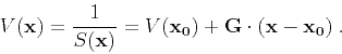 |
(2) |
It is convenient to change the parameterization of the ray tracing
system, with parameter  defined by equation (3) below:
and consider the one-point ray tracing problem with the initial conditions
 and
and
 .
.
- Show that the solution of
equation (3) for the constant gradient of velocity is
 |
(6) |
and express velocity along the ray as a function of
 ,
,  , and :
 |
(7) |
- Let
 . Using
the chain rule, find the expression for
. Using
the chain rule, find the expression for
 |
(8) |
and solve it to show it that
 |
(9) |
and
 |
(10) |
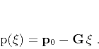
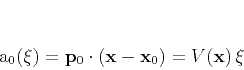
- One way to seek the solution for the one-point ray tracing
problem is to look for scalars
 and
and  in the representation
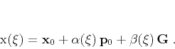 |
(11) |
Under what condition does the linear system of equations
have a unique solution for and ? Solve the system to
find and and obtain an analytical expression for
the ray trajectory
 .
.
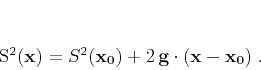
- Express the squared distance between the ray end points
in terms of , , and .
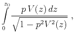
- In the two-point problem, the unknown
parameters are
 and .
Express
from your
equation (7) and substitute it into your
equation (14). Solve for .
and .
Express
from your
equation (7) and substitute it into your
equation (14). Solve for .
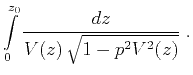
- Finally, use and
expressed in terms of
 ,
,
,
,
 , and
, and  and
substitute them into the one-point traveltime solution obtained by
integrating equation (5)
and
substitute them into the one-point traveltime solution obtained by
integrating equation (5)![[*]](icons/footnote.png)
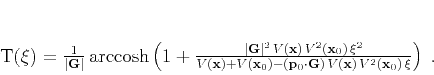 |
(15) |
Your result will be the analytical two-point
traveltime
 |
|
 |
(16) |
- In class, we discussed the hyperbolic traveltime approximation for normal moveout
 |
(17) |
More accurate approximations, involving additional parameters, are possible.
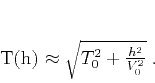
- Consider the following three-parameter approximation
 |
(18) |
where  is the so-called ``heterogeneity'' parameter.
Evaluate parameter in terms of the velocity  and the reflector depth
  .
.
 |
(19) |
by expanding
equation (18) in a Taylor series around the zero offset
 and comparing it with the corresponding Taylor series of the exact
traveltime. The exact traveltime is given by the parametric equations
and comparing it with the corresponding Taylor series of the exact
traveltime. The exact traveltime is given by the parametric equations
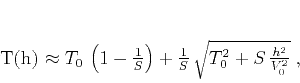
- Let
 . Show that the function
  can be approximated to the same accuracy by
 |
(22) |
Find  ,
,  , and
, and  .
.
Next: Computational part 1
Up: Homework 2
Previous: Homework 2
2019-09-26