|
|
|
|
GEO 365N/384S Seismic Data Processing Computational Assignment 4 |
Next, we return to processing the Teapot Dome data. Our task is to estimate the surface-consistent amplitude normalization, similar to how it was done with the two previous datasets.
scons -cto remove (clean) previously generated files.
scons sint.view
|
|---|
|
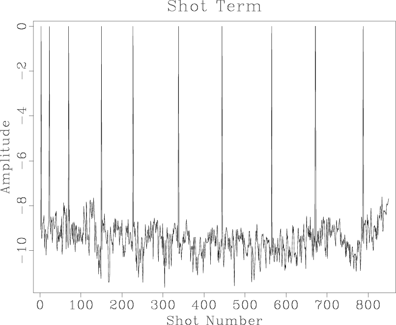
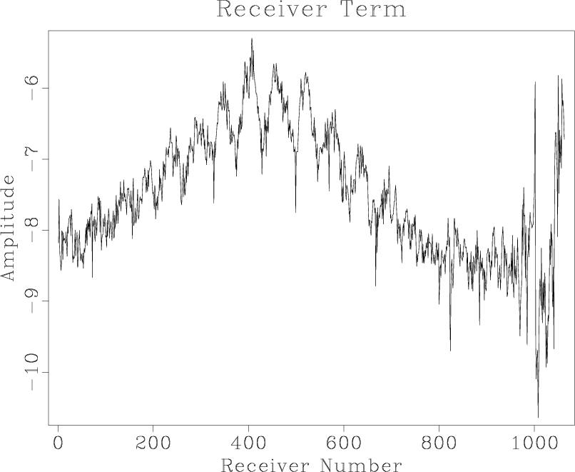
tshot,treceiver
Figure 14. Estimated shot and receiver surface-consistent amplitude terms for the Teapot Dome dataset. |
|
|
|
|---|
|
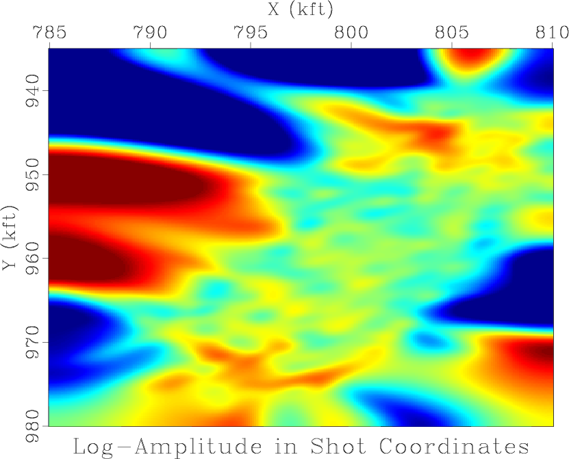
sint
Figure 15. Surface-consistent amplitude interpolated using the shot coordinates. |
|
|
from rsf.proj import *

# Download Teapot Dome field data
#Fetch('npr3_field.sgy','teapot',
#      server='http://s3.amazonaws.com',top='')
Fetch('npr3_field.sgy','TeapotDome3D',
      top='/home/p1/seismic_datasets/SeismicProcessingClass',
      server='local')

# Convert to RSF
Flow('traces header header.asc','npr3_field.sgy',
     'segyread tfile=${TARGETS[1]} hfile=${TARGETS[2]}')

# Seismic data corresponds to trid=1
Flow('trid','header','headermath output=trid | mask min=1 max=1')

# Average trace amplitude
Flow('arms','traces trid',
     '''
     mul $SOURCE | headerwindow mask=${SOURCES[1]} |
     stack axis=1 | math output="log(input)"
     ''')
Flow('theader','header trid','headerwindow mask=${SOURCES[1]}')

# shot/receiver indeces: fldr and tracf
Flow('index','theader','window n1=2 f1=2 | transp')

prog = Program('../alaska/surface-consistent.c')
sc = str(prog[0])

Flow('model',['arms','index',sc],
     '${SOURCES[2]} index=${SOURCES[1]} verb=y')

Flow('sc',['arms','index',sc,'model'],
     '''
     conjgrad ${SOURCES[2]} index=${SOURCES[1]}
     mod=${SOURCES[3]} niter=50
     ''')

Result('tshot','sc',
       '''
       window n1=850 | put o1=1 d1=1 |
       graph title="Shot Term"
       label1="Shot Number" unit1= label2=Amplitude unit2=
       ''')
Result('treceiver','sc',
       '''
       window f1=850 n1=1063 | put o1=1 d1=1 |
       graph title="Receiver Term"
       label1="Receiver Number" unit1= label2=Amplitude unit2=
       ''')

# Surface-consistent Log Amplitude for each trace
Flow('scarms',['sc','index',sc],
     '${SOURCES[2]} index=${SOURCES[1]} adj=n')

# Interpolate to a regular grid

# !!!! MODIFY BELOW !!!

# Using sx and sy
Flow('scoord','theader',
     'window n1=2 f1=21 | dd type=float | scale dscale=1e-6')
Flow('sint','scarms scoord',
     '''
     nnshape coord=${SOURCES[1]} rect1=10 rect2=10
     o1=785 d1=0.1 n1=251 o2=935 d2=0.1 n2=451 niter=10
     ''')
Result('sint',
       '''
       grey color=j title="Log-Amplitude in Shot Coordinates"
       transp=n label1=X label2=Y unit1=kft unit2=kft
       bias=-17 clip=3
       ''')

End()
|
|
|
|
|
GEO 365N/384S Seismic Data Processing Computational Assignment 4 |