|
|
|
|
GEO 365N/384S Seismic Data Processing Computational Assignment 4 |
In the next part of the assignment, we will take a step back in processing the Viking Graben dataset and use the original unprocessed data.
scons -cto remove (clean) previously generated files.
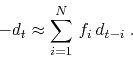
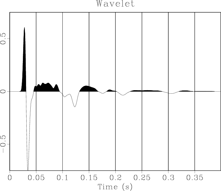
scons wavelet.viewAs typical for marine data, the wavelet, instead of being a perfect impulse, contains additional components (bubble pulse, ghost reflection, etc.) The wavelet spectrum, displayed with
scons spectrum.viewshows frequencies missing from the ideal flat response.
|
|---|
|
wavelet,spectrum
Figure 9. Far-field wavelet (a) and its Fourier spectrum (b). |
|
|
As in the surface-consistent problem, the least-squares solution can be found using a generic conjugate-gradient program, which simply requires an implementation of the convolution operator in the right-hand side of equation (3) and its adjoint. An implementation is provided in the convolve.c program.
/* Match filtering */
#include <rsf.h>

int main(int argc, char* argv[])
{
    bool adj;
    int n1, n2, i1, i2, i, j, nf;
    float *data, *target, *filter;
    sf_file inp, out, other;

    sf_init(argc,argv);
    inp = sf_input("in");
    out = sf_output("out");
    other = sf_input("data");

    if (!sf_getbool("adj",&adj)) adj=false;
    /* adjoint flag */

    if (adj) {
	/* input data, output filter */
	if (!sf_histint(inp,"n1",&n1)) sf_error("No n1=");
	if (!sf_histint(inp,"n2",&n2)) sf_error("No n2=");
	if (!sf_getint("nf",&nf)) sf_error("Need nf=");
	/* filter size */

	sf_putint(out,"n1",nf);
	sf_putint(out,"n2",1);
    } else {
	/* input filter, output data */
	if (!sf_histint(inp,"n1",&nf)) sf_error("No n1=");
	if (!sf_histint(other,"n1",&n1)) sf_error("No n1=");
	if (!sf_histint(other,"n2",&n2)) sf_error("No n2=");

	sf_fileflush(out,other);  /* copy data dimensions */
    }

    filter = sf_floatalloc(nf);
    target = sf_floatalloc(n1);
    data = sf_floatalloc(n1);

    if (adj) {
	for (i=0; i < nf; i++) filter[i]=0.0f;
    } else {
	sf_floatread(filter,nf,inp);
    }

    for (i2=0; i2 < n2; i2++) {
	sf_floatread(data,n1,other);

	if (adj) {
	    sf_floatread(target,n1,inp);
	} else {
	    for (i1=0; i1 < n1; i1++) target[i1] = 0.0f;
	}

	for (i1=0; i1 < n1; i1++) {
	    for (i=0; i < nf; i++) {

		j=i1-i-1;

		/* zero value boundary conditions */
		if (j < 0 || j >= n1) continue;

		if (adj) {
		    filter[i] += data[j]*target[i1];
		} else {
		    target[i1] += data[j]*filter[i];
		}
	    }
	}

	if (!adj) sf_floatwrite(target,n1,out);
    }

    if (adj) sf_floatwrite(filter,nf,out);

    exit(0);
}
|
To test the program using the generic dot-product test, you can run
scons filter0.rsf wavelet4.rsf
scons convolve.exe
sfdottest ./convolve.exe nf=100 mod=filter0.rsf dat=wavelet4.rsf
The test should show pairs of numbers matching to several significant digits.
To run the least-squares inversion and to estimate the filter, run
scons filter.view
|
|---|
|
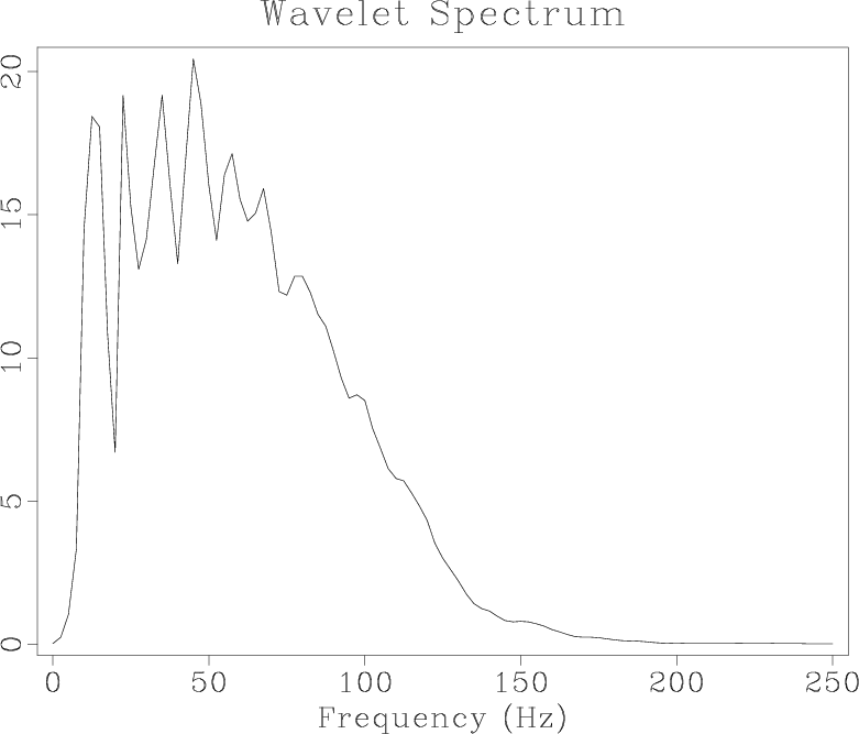
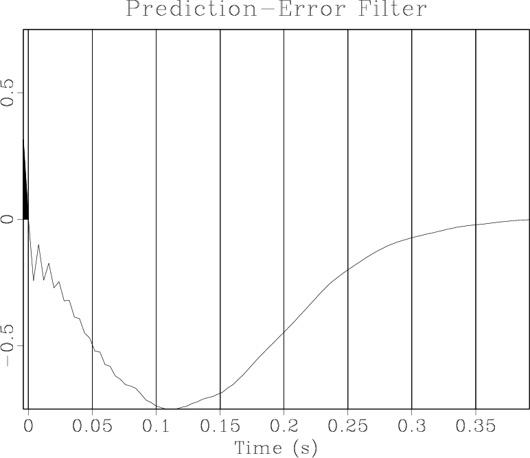
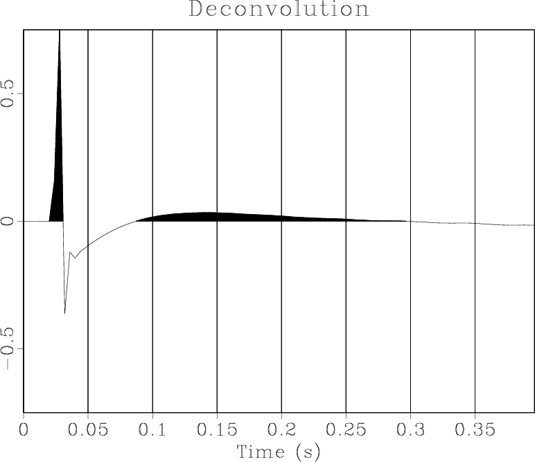
filter,wdecon
Figure 10. Estimated prediction-error filter (a) and the result of wavelet deconvolution (b). |
|
|
Although deconvolution applied to the wavelet (Figure 10b) does not produce a perfect spike, it improves the spikiness of the wavelet and its spectral content.
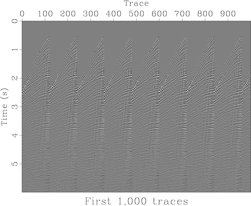
scons viking1000.viewto extract and display the first 1,000 traces from the Viking Graben dataset (Figure 11.) Run
scons decon1000.viewto display the result of deconvolution (Figure 12.)
|
|---|
|
viking1000
Figure 11. First 1,000 traces from the Viking Graben dataset. |
|
|

|
|---|
|
decon1000
Figure 12. Viking Graben traces after deconvolution. |
|
|
To apply deconvolution to the whole dataset, run
scons decon.rsf
 with something like
 and process the data quickly in parallel.
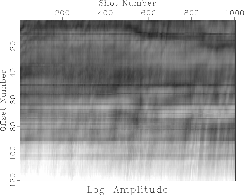
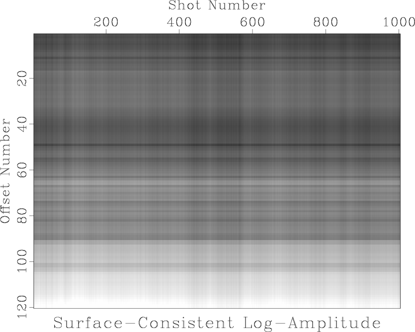
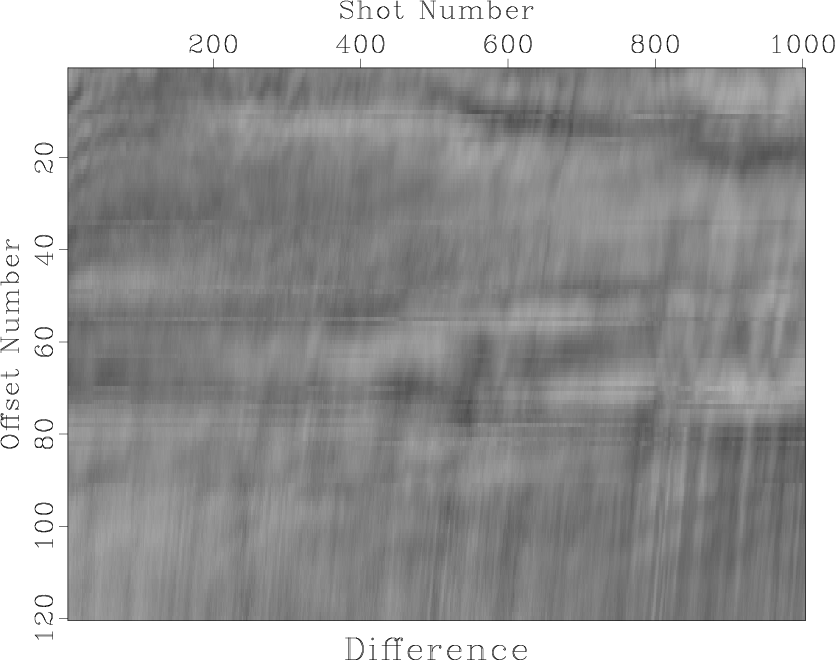
scons vadiff.viewCan you notice remaining stripes in the difference? Which of the four terms in equation (2) are the stripes coming from?

|
|---|
|
varms,vscarms,vadiff
Figure 13. Trace amplitudes from the Viking Graben dataset. (a) Initial. (b) Estimated surface-consistent. (c) Difference. |
|
|
from rsf.proj import *
# Download Viking Graben data
#Fetch('seismic.segy','viking')
Fetch('seismic.segy','VikingGrabbenLine12',
top='/home/p1/seismic_datasets/SeismicProcessingClass',
server='local')
# Convert from SEGY to RSF
Flow('viking tviking viking.asc viking.bin','seismic.segy',
'''
segyread tfile=${TARGETS[1]}
hfile=${TARGETS[2]} bfile=${TARGETS[3]}
''')
# Far-field wavelet
Fetch('FarField.dat','Mobil_Avo_Viking_Graben_Line_12',
top='open.source.geoscience/open_data',
server='http://s3.amazonaws.com')
# Convert from ASCII to RSF
Flow('wavelet','FarField.dat',
'''
echo in=$SOURCE data_format=ascii_float n1=500 o1=0 d1=0.0008
label1=Time unit1=s n2=1 | dd form=native
''')
Result('wavelet','wiggle poly=y title=Wavelet pclip=100')
Result('spectrum','wavelet',
'''
spectra | window max1=250 |
graph title="Wavelet Spectrum"
''')
# Subsample to data sampling
Flow('wavelet4','wavelet','window j1=5 | pad n1=1500')
prog = Program('convolve.c')
convolve = str(prog[0])
# Estimate PEF by iterative least-squares inversion
Flow('filter0',None,'spike n1=100 k1=1')
Flow('filter',['wavelet4',convolve,'filter0'],
'''
conjgrad ./${SOURCES[1]} nf=100 data=${SOURCES[0]}
niter=100 mod=${SOURCES[2]}
''')
Result('filter','filter filter0',
'''
pad beg1=1 | window n1=100 |
scale axis=-1 | add ${SOURCES[1]} |
wiggle poly=y title="Prediction-Error Filter" pclip=100
''')
# Wavelet deconvolution
Flow('wdecon',['filter','wavelet4',convolve],
'''
./${SOURCES[2]} data=${SOURCES[1]} adj=n |
add ${SOURCES[1]} scale=-1,1 | window n1=100
''')
Result('wdecon','wiggle poly=y title=Deconvolution pclip=100')
# Apply to the first 1000 traces
Flow('viking1000','viking','window n2=1000')
Result('viking1000','pow pow1=2 | grey title="First 1,000 traces" ')
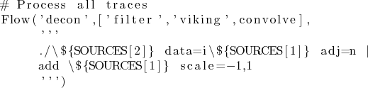
Flow('decon1000',['filter','viking1000',convolve],
'''
./${SOURCES[2]} data=${SOURCES[1]} adj=n |
add ${SOURCES[1]} scale=-1,1
''')
Result('decon1000',
'pow pow1=2 | grey title=Deconvolution ')
# Process all traces
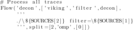
Flow('decon',['filter','viking',convolve],
'''
./${SOURCES[2]} data=${SOURCES[1]} adj=n |
add ${SOURCES[1]} scale=-1,1
''')
# Average trace amplitude
Flow('arms','decon',
'mul $SOURCE | stack axis=1 | math output="log(input)" ')
# shot/offset indeces: fldr and tracf
Flow('index','tviking','window n1=2 f1=2 | transp')
def plot(title,bias=5):
return '''
spray axis=1 n=1 |
intbin head=${SOURCES[1]} yk=fldr xk=tracf | window |
grey title="%s" label2="Shot Number" unit2=
label1="Offset Number" unit1= bias=%d clip=3
''' % (title,bias)
# Display in shot/offset coordinates
Result('varms','arms tviking',plot('Log-Amplitude'))
prog = Program('../alaska/surface-consistent.c')
sc = str(prog[0])
Flow('model',['arms','index',sc],
'${SOURCES[2]} index=${SOURCES[1]} verb=y')
Flow('sc',['arms','index',sc,'model'],
'''
conjgrad ${SOURCES[2]} index=${SOURCES[1]}
mod=${SOURCES[3]} niter=10
''')
Result('vshot','sc',
'''
window n1=1000 | put o1=1 d1=1 |
graph title="Shot Term"
label1="Shot Number" unit1= label2=Amplitude unit2=
''')
Result('voffset','sc',
'''
window f1=1000 n1=120 | put o1=1 d1=1 |
graph title="Offset Term"
label1="Offset Number" unit1= label2=Amplitude unit2=
''')
Flow('scarms',['sc','index',sc],
'${SOURCES[2]} index=${SOURCES[1]} adj=n')
Result('vscarms','scarms tviking',
plot('Surface-Consistent Log-Amplitude'))
Flow('adiff','arms scarms','add scale=1,-1 ${SOURCES[1]}')
Result('vadiff','adiff tviking',plot('Difference',0))
End()
|
|
|
|
|
GEO 365N/384S Seismic Data Processing Computational Assignment 4 |