|
|
|
|
Homework 2 |
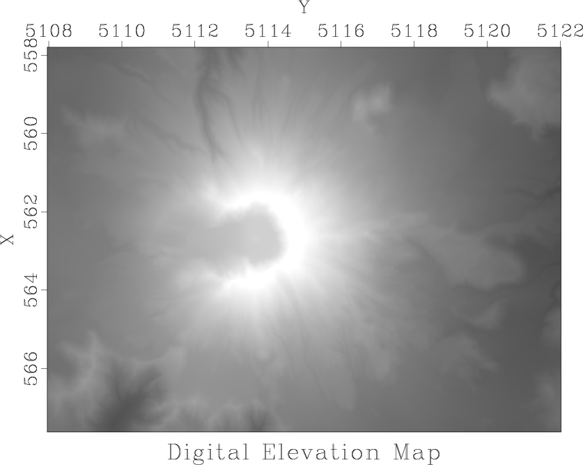
In this part of the assignment, we will use a digital elevation map of the Mount St. Helens area, shown in Figure 3.
|
data
Figure 3. Digital elevation map of Mount St. Helens area. |
|
|---|---|
|
|
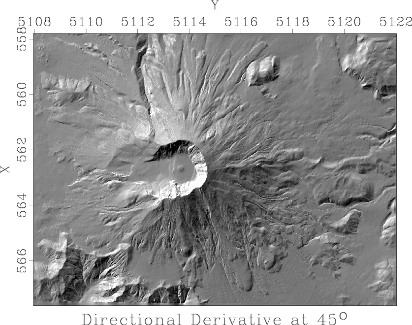
Figure 4 shows a directional derivative, a digital approximation to
|
der
Figure 4. Directional derivative of elevation. |
|
|---|---|
|
|
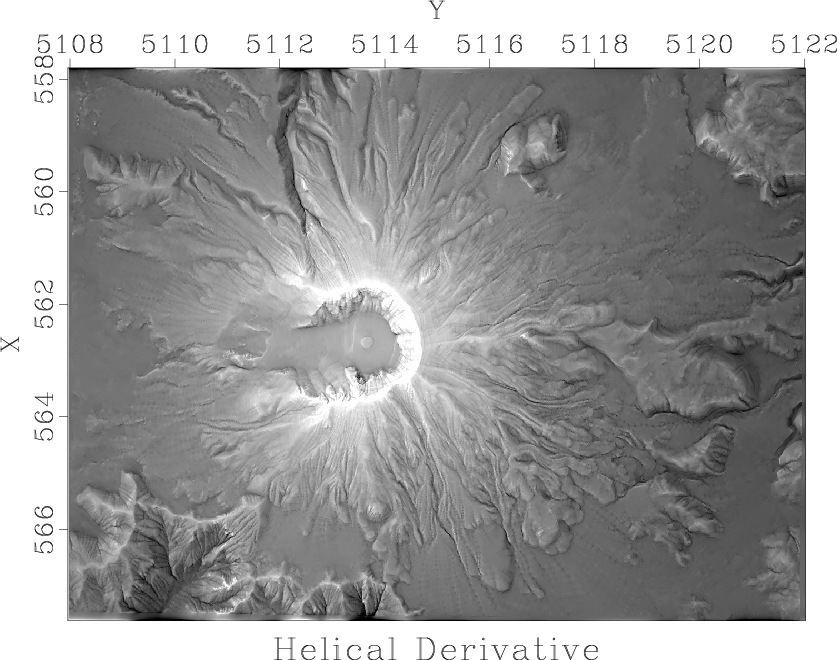
Figure 5 shows an application of helical
derivative, a filter designed by spectral factorization of the
Laplacian filter
|
helder
Figure 5. Helix derivative of elevation. |
|
|---|---|
|
|
scons viewto reproduce the figures on your screen.
scons der.view
from rsf.proj import *
import math

# Download data
txt = 'st-helens_after.txt'
Fetch(txt,'data',
      server='https://raw.githubusercontent.com',
      top='agile-geoscience/notebooks/master')
Flow('data.asc',txt,'/usr/bin/tail -n +6')

# Convert to RSF format
Flow('data','data.asc',
     '''
     echo in=$SOURCE data_format=ascii_float
     label=Elevation unit=m
     n1=979  o1=557.805  d1=0.010030675 label1=X
     n2=1400 o2=5107.965 d2=0.010035740 label2=Y |
     dd form=native |
     clip2 lower=0 | lapfill grad=y niter=200
     ''')

Result('data','grey title="Digital Elevation Map" allpos=y')

# Vertical and horizontal derivatives
Flow('der1','data','igrad')
Flow('der2','data','transp | igrad | transp')

ders = []
for alpha in range(0,360,15):
    der = 'der%d' % alpha

    # Directional derivative
    Flow(der,'der1 der2',
         '''
         add ${SOURCES[1]} scale=%g,%g
         ''' % (math.cos(alpha*math.pi/180),
                math.sin(alpha*math.pi/180)))
    ders.append(der)

Flow('ders',ders,
     '''
     cat axis=3 ${SOURCES[1:%d]} |
     put o3=0 d3=15
     ''' % len(ders))
Plot('ders','grey gainpanel=all wanttitle=n',view=1)

# !!! MODIFY BELOW !!!
alpha=45

Result('der','der%d' % alpha,
       '''
       grey title="Directional Derivative at %gô_"
       ''' % alpha)

# Laplacian filter on a helix (!!! MODIFY !!!)

Flow('slag0.asc',None,
     '''echo 1 1000 n1=2 n=1000,1000
     data_format=ascii_int in=$TARGET
     ''')
Flow('slag','slag0.asc','dd form=native')

Flow('ss0.asc','slag',
     '''echo -1 -1 a0=2 n1=2
     lag=$SOURCE in=$TARGET data_format=ascii_float''')
Flow('ss','ss0.asc','dd form=native')

# Wilson-Burg factorization

na=50 # filter length

lags = list(range(1,na+1)) + list(range(1002-na,1002))

Flow('alag0.asc',None,
     '''echo %s n=1000,1000 n1=%d in=$TARGET
     data_format=ascii_int
     ''' % (' '.join([str(x) for x in lags]),2*na))
Flow('alag','alag0.asc','dd form=native')

Flow('hflt hlag','ss alag',
     'wilson lagin=${SOURCES[1]} lagout=${TARGETS[1]}')

# Helical derivative

Flow('helder','data hflt hlag','helicon filt=${SOURCES[1]}')
Result('helder','grey mean=y title="Helical Derivative" ')

def plotfilt(title):
    return '''
    window n1=11 n2=11 f1=50 f2=50 |
    grey wantaxis=n title="%s" pclip=100
    crowd=0.85 screenratio=1
    ''' % title

# Laplacian impulse response
Flow('spike',None,'spike n1=111 n2=111 k1=56 k2=56')
Flow('imp0','spike ss','helicon filt=${SOURCES[1]} adj=0')
Flow('imp1','spike ss','helicon filt=${SOURCES[1]} adj=1')
Flow('imp','imp0 imp1','add ${SOURCES[1]}')
Plot('imp',plotfilt('(a) Laplacian'))

# Test factorization
Flow('fac0','imp hflt',
     'helicon filt=${SOURCES[1]} adj=0 div=1')
Flow('fac1','imp hflt',
     'helicon filt=${SOURCES[1]} adj=1 div=1')
Plot('fac0',plotfilt('(b) Laplacian/Factor'))
Plot('fac1',plotfilt('(c) Laplacian/Factor'))
Flow('fac','fac0 hflt',
     'helicon filt=${SOURCES[1]} adj=1 div=1')
Plot('fac',plotfilt('(d) Laplacian/Factor/Factor'))

Result('laplace','imp fac0 fac1 fac','TwoRows',
       vppen='gridsize=5,5 xsize=11 ysize=11')

End()
|
|
|
|
|
Homework 2 |