|
|
|
|
Homework 2 |
|
bay
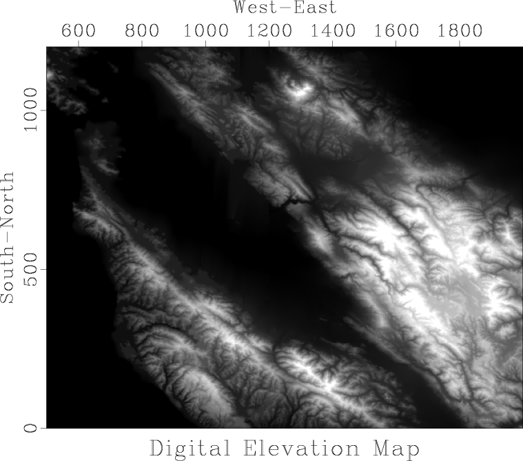
Figure 1. Digital elevation map of the San Francisco Bay Area. |
|
|---|---|
|
|
We return the digital elevation map of the San Francisco Bay Area, shown in Figure ![]() .
.
In this exercise, we will separate the data into ``signal'' and ``noise'' by applying running mean and median filters. The result of applying a running median filter is shown in Figure 2. Running median effectively smooths the data by removing local outliers.


|
|---|
|
ave,res
Figure 2. Data separated into signal (a) and noise (b) by applying a running median filter. |
|
|
The algorithm is implemented in programs below.
/* Apply running mean or median filter */
#include <rsf.h>
static float slow_median(int n, float* list)
/* find median by slow sorting, changes list */
{
int k, k2;
float item1, item2;
for (k=0; k < n; k++) {
item1 = list[k];
/* assume everything up to k is sorted */
for (k2=k; k2 > 0; k2-) {
item2 = list[k2-1];
if (item1 >= item2) break;
list[k2] = item2;
}
list[k2] = item1;
}
return list[n/2];
}
int main(int argc, char* argv[])
{
int w1, w2, nw, s1,s2, j1,j2, i1,i2,i3, n1,n2,n3;
char *how;
float **data, **signal, **win;
sf_file in, out;
sf_init (argc,argv);
in = sf_input("in");
out = sf_output("out");
/* get data dimensions */
if (!sf_histint(in,"n1",&n1)) sf_error("No n1=");
if (!sf_histint(in,"n2",&n2)) sf_error("No n2=");
n3 = sf_leftsize(in,2);
/* input and output */
data = sf_floatalloc2(n1,n2);
signal = sf_floatalloc2(n1,n2);
if (!sf_getint("w1",&w1)) w1=5;
if (!sf_getint("w2",&w2)) w2=5;
/* sliding window width */
nw = w1*w2;
win = sf_floatalloc2(w1,w2);
how = sf_getstring("how");
/* what to compute
(fast median, slow median, mean) */
if (NULL == how) how="fast";
for (i3=0; i3 < n3; i3++) {
/* read data plane */
sf_floatread(data[0],n1*n2,in);
for (i2=0; i2 < n2; i2++) {
s2 = SF_MAX(0,SF_MIN(n2-w2,i2-w2/2-1));
for (i1=0; i1 < n1; i1++) {
s1 = SF_MAX(0,SF_MIN(n1-w1,i1-w1/2-1));
/* copy window */
for (j2=0; j2 < w2; j2++) {
for (j1=0; j1 < w1; j1++) {
win[j2][j1] = data[s2+j2][s1+j1];
}
}
switch (how[0]) {
case 'f': /* fast median */
signal[i2][i1] =
sf_quantile(nw/2,nw,win[0]);
break;
case 's': /* slow median */
signal[i2][i1] =
slow_median(nw,win[0]);
break;
case 'm': /* mean */
/* !!! ADD CODE !!! */
break;
default:
sf_error("Unknown method "%s"",how);
break;
}
}
}
/* write out */
sf_floatwrite(signal[0],n1*n2,out);
}
exit(0);
}
|
#!/usr/bin/env python

import sys
import numpy as np
import m8r

def slow_median(data):
    'find median by slow sorting, changes data'

    n = len(data)
    for k in range(n):
        item1 = data[k]

        # assume everything up to k is sorted
        for k2 in range(k,-1,-1):
            item2 = data[k2-1]
            if item1 >= item2:
                break
            data[k2] = item2

        data[k2] = item1

    return data[n/2]

# initialization
par = m8r.Par()
inp = m8r.Input()
out = m8r.Output()

# get data dimensions
n1 = inp.int('n1')
n2 = inp.int('n2')
n3 = inp.leftsize(2)

# input and output
data = np.zeros([n2,n1],'f')
signal = np.zeros([n2,n1],'f')

# sliding window
w1 = par.int('w1',5)
w2 = par.int('w2',5)

nw = w1*w2
win = np.zeros([w2,w1],'f')

how = par.string('how','fast')
# what to compute
# (fast median, slow median, mean)

for i3 in range(n3):
    # read data plane
    inp.read(data)

    for i2 in range(n2):
        sys.stderr.write("%d of %d" % (i2,n2))
        s2 = max(0,min(n2-w2,i2-w2/2-1))
        for i1 in range(n1):
            s1 = max(0,min(n1-w1,i1-w1/2-1))

	    # copy window
            win = data[s2:s2+w2,s1:s1+w1]

            if how[0] == 'f': # fast median
                signal[i2,i1] = np.median(win)
            elif how[0] == 's': # slow median
                signal[i2,i1] = slow_median(win.flatten())
            elif how[0] == 'm': # mean
                # !!! ADD CODE !!!
                pass
            else:
                sys.stderr.write(
                    "Unknown method "%s"" % how)
                sys.exit(1)
    sys.stderr.write("")
    # write out
    out.write(signal)

sys.exit(0)
|
scons viewto reproduce the figures on your screen.
scons time.vplto display a figure that compares the efficiency of running median computations using the slow sorting from function median in program run.c (or run.py) and the fast median algorithm. Your goal is to make the algorithm even faster. You may consider parallelization, reusing previous windows, other fast sorting strategies, etc.
from rsf.proj import *

# Download data
Fetch('bay.h','bay')

# Convert format
Flow('bay','bay.h',
     '''
     dd form=native |
     window f2=500 n2=1500
     ''')

# Display
def plot(title):
    return '''
    grey allpos=y title="%s" yreverse=n
    label1=South-North label2=West-East
    screenratio=0.8
    ''' % title

Result('bay',plot('Digital Elevation Map'))

# Program for running average
run = Program('run.c')

# COMMENT ABOVE AND UNCOMMENT BELOW IF YOU WANT TO USE PYTHON
# run = Command('run.exe','run.py','cp $SOURCE $TARGET')
# AddPostAction(run,Chmod(run,0o755))

w = 30

# !!! CHANGE BELOW !!!
Flow('ave','bay %s' % run[0],
     './${SOURCES[1]} w1=%d w2=%d how=fast' % (w,w))
Result('ave',plot('Signal'))

# Difference
Flow('res','bay ave','add scale=1,-1 ${SOURCES[1]}')
Result('res',plot('Noise') + ' allpos=n')

#############################################################

import sys

if sys.platform=='darwin':
     gtime = WhereIs('gtime')
     if not gtime:
          print("For computing CPU time, install gtime.")
else:
     gtime = WhereIs('gtime') or WhereIs('time')

# slow or fast
for case in ('fast','slow'):

    ts = []
    ws = []

    time = 'time-' + case
    wind = 'wind-' + case

    # loop over window size
    for w in range(3,16,2):
        itime = '%s-%d' % (time,w)
        ts.append(itime)

        iwind = '%s-%d' % (wind,w)
        ws.append(iwind)

        # measure CPU time
        Flow(iwind,None,'spike n1=1 mag=%d' % (w*w))
        Flow(itime,'bay %s' % run[0],
             '''
             ( (%s -f "%%S %%U"
             ./${SOURCES[1]} < ${SOURCES[0]}
              w1=%d w2=%d how=%s > /dev/null ) 2>&1 )
              > time.out &&
             (tail -1 time.out;
              echo in=time0.asc n1=2 data_format=ascii_float)
              > time0.asc &&
             dd form=native < time0.asc | stack axis=1 norm=n
             > $TARGET &&
             /bin/rm time0.asc time.out
             ''' % (gtime,w,w,case),stdin=0,stdout=-1)

    Flow(time,ts,'cat axis=1 ${SOURCES[1:%d]}' % len(ts))
    Flow(wind,ws,'cat axis=1 ${SOURCES[1:%d]}' % len(ws))

    # complex numbers for plotting
    Flow('c'+time,[wind,time],
         '''
         cat axis=2 ${SOURCES[1]} |
         transp |
         dd type=complex
         ''')

# Display CPU time
Plot('time','ctime-fast ctime-slow',
     '''
     cat axis=1 ${SOURCES[1]} | transp |
     graph dash=0,1 wanttitle=n
     label2="CPU Time" unit2=s
     label1="Window Size" unit1=
     ''',view=1)

End()
|
|
|
|
|
Homework 2 |