|
|
|
|
Nonstationarity: patching |
Normally, the number of filter coefficients is many fewer
than the number of data points,
but here we have very many more.
Indeed, there are na times more.
Variable filters require na times more memory than the data itself.
To make the nonstationary helix code more practical,
we now require the filters to be constant in patches.
The data type for nonstationary filters
(which are constant in patches)
is introduced in module
nhelix, which is a simple modification of module
helix ![]() .
.
typedef struct nhelixfilter {
    int np;
    sf_filter* hlx;
    bool* mis;
    int *pch;
} *nfilter;
|
nfilter createnhelix(int dim     /* number of dimensions */,
		     int *nd     /* data size [dim] */,
		     int *center /* filter center [dim] */,
		     int *gap    /* filter gap [dim] */,
		     int *na     /* filter size [dim] */,
		     int *pch    /* patching [product(nd)] */)
/*< allocate and output a non-stationary filter >*/
{
    nfilter nsaa;
    sf_filter aa;
    int n123, np, ip, *nh, i;

    aa = createhelix(dim, nd, center, gap, na);

    n123=1;
    for (i=0; i < dim; i++) {
	n123 *= nd[i];
    }
    np = pch[0];
    for (i=0; i < n123; i++) {
	if (pch[i] > np) np=pch[i];
    }
    np++;

    nh = sf_intalloc(np);
    for (ip=0; ip < np; ip++) {
	nh[ip] = aa->nh;
    }
    nsaa = nallocate(np, n123, nh, pch);
    for (ip=0; ip < np; ip++) {
	for (i=0; i < aa->nh; i++) {
	    nsaa->hlx[ip]->lag[i] = aa->lag[i];
	}
	nbound(ip, dim, nd, na, nsaa);
    }

    sf_deallocatehelix(aa);

    return nsaa;
}
|
Finally, we are ready for the convolution operator.
The operator nhconest ![]() allows for a different filter in each patch.
allows for a different filter in each patch.
    for (iy=0; iy < ny; iy++) {
	if (aa->mis[iy]) continue;

        ip = aa->pch[iy];
	lag = aa->hlx[ip]->lag;
	na = aa->hlx[ip]->nh;

        for (ia=0; ia < na; ia++) {
	    ix = iy - lag[ia];
	    if (ix < 0) continue;

	    if (adj) {
		a[ia+nhmax*ip] += y[iy] * x[ix];
	    } else {
		y[iy] += a[ia+nhmax*ip] * x[ix];
	    }
        }
    }
|
Because of the massive increase in the number of filter coefficients,
allowing these many filters
takes us from overdetermined to very undetermined.
We can estimate all these filter coefficients
by the usual deconvolution fitting goal (![]() )
)
| (21) |
Experience with missing data in Chapter ![]() shows that when the roughening operator
shows that when the roughening operator ![]() is a differential operator,
the number of iterations can be large.
We can speed the calculation immensely by ``preconditioning''.
Define a new variable
is a differential operator,
the number of iterations can be large.
We can speed the calculation immensely by ``preconditioning''.
Define a new variable ![]() by
by
![]() and insert it into (22) to get
the equivalent preconditioned system of goals.
and insert it into (22) to get
the equivalent preconditioned system of goals.
The fitting (23) uses the operator
![]() .
For
.
For ![]() we can use subroutine
nhconest()
we can use subroutine
nhconest() ![]() ;
for the smoothing operator
;
for the smoothing operator
![]() we can use nonstationary
polynomial division
with operator npolydiv():
we can use nonstationary
polynomial division
with operator npolydiv():
    for (id=0; id < nd; id++) {
	tt[id] = adj? yy[id]: xx[id];
    }

    if (adj) {
        for (iy=nd-1; iy >= 0; iy-) {
	    ip = aa->pch[iy];
	    lag = aa->hlx[ip]->lag;
	    flt = aa->hlx[ip]->flt;
	    na = aa->hlx[ip]->nh;
	    for (ia=0; ia < na; ia++) {
		ix = iy - lag[ia];
		if (ix < 0)  continue;
		tt[ix] -=  flt[ia] * tt[iy];
	    }
	}
	for (id=0; id < nd; id++) {
	    xx[id] += tt[id];
	}
    } else {
        for (iy=0; iy < nd; iy++) {
	    ip = aa->pch[iy];
	    lag = aa->hlx[ip]->lag;
	    flt = aa->hlx[ip]->flt;
	    na = aa->hlx[ip]->nh;
	    for (ia=0; ia < na; ia++) {
		ix = iy - lag[ia];
		if (ix < 0)  continue;
		tt[iy] -=  flt[ia] * tt[ix];
	    }
	}
	for (id=0; id < nd; id++) {
	    yy[id] += tt[id];
        }
    }
|
Now we have all the pieces we need.
As we previously estimated stationary filters with
the module pef ![]() ,
now we can estimate nonstationary PEFs with
the module npef
,
now we can estimate nonstationary PEFs with
the module npef ![]() .
The steps are hardly any different.
.
The steps are hardly any different.
void find_pef(int nd     /* data size */,
	      float *dd  /* data */,
	      nfilter aa /* estimated filter */,
	      nfilter rr /* regularization filter */,
	      int niter  /* number of iterations */,
	      float eps  /* regularization parameter */,
	      int nh     /* filter size */)
/*< estimate non-stationary PEF >*/
{
    int ip, ih, na, np, nr;
    float *flt;

    np = aa->np;
    nr = np*nh;
    flt = sf_floatalloc(nr);

    nhconest_init(dd, aa, nh);
    npolydiv2_init( nr, rr);

    sf_solver_prec(nhconest_lop, sf_cgstep, npolydiv2_lop,
		   nr, nr, nd, flt, dd, niter, eps, "end");
    sf_cgstep_close();
    npolydiv2_close();

    for (ip=0; ip < np; ip++) {
	na = aa->hlx[ip]->nh;
	for (ih=0; ih < na; ih++) {
	    aa->hlx[ip]->flt[ih] = -flt[ip*nh + ih];
	}
    }

    free(flt);
}
|
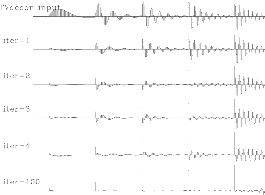
Figure 15 shows a synthetic data example using these programs.
As we hope for deconvolution, events are compressed.
The compression is fairly good, even though each event has
a different spectrum.
What is especially pleasing is that satisfactory results
are obtained in truly small numbers of iterations (about three).
The example is for two free filter coefficients
![]() per output point.
The roughening operator
per output point.
The roughening operator ![]() was taken to be
was taken to be ![]() which was factored into
causal and anticausal finite difference.
which was factored into
causal and anticausal finite difference.
|
|---|
|
tvdecon
Figure 15. Time variable deconvolution with two free filter coefficients and a gap of 6. |
|
|
I hope also to find a test case with field data, but experience in seismology is that spectral changes are slow, which implies unexciting results. Many interesting examples should exist in two- and three-dimensional filtering, however, because reflector dip is always changing and that changes the spatial spectrum.
In multidimensional space, the smoothing filter
![]() can be chosen with interesting directional properties.
Sergey, Bob, Sean and I have joked about this code being
the ``double helix'' program because there are two multidimensional
helixes in it, one the smoothing filter, the other the deconvolution filter.
Unlike the biological helixes, however, these two helixes
do not seem to form a symmetrical pair.
can be chosen with interesting directional properties.
Sergey, Bob, Sean and I have joked about this code being
the ``double helix'' program because there are two multidimensional
helixes in it, one the smoothing filter, the other the deconvolution filter.
Unlike the biological helixes, however, these two helixes
do not seem to form a symmetrical pair.
|
|
|
|
Nonstationarity: patching |
