|
|
|
|
Model fitting by least squares |
Equation (1) gives us one way to divide by zero.
Another way is stated by the equation
Both divisions,
equation (1) and
equation (6),
irritate us by requiring us to specify a parameter,
but for the latter, the parameter has a clear meaning.
In the latter case we smooth a spectrum with a smoothing
window of width, say ![]() which this corresponds inversely to a time interval over which we smooth.
Choosing a numerical value for
which this corresponds inversely to a time interval over which we smooth.
Choosing a numerical value for ![]() has not such a simple interpretation.
has not such a simple interpretation.
We jump from simple mathematical theorizing
towards a genuine practical application when I grab some real data,
a function of time and space from another textbook.
Let us call this data ![]() and its 2-D Fourier transform
and its 2-D Fourier transform
![]() .
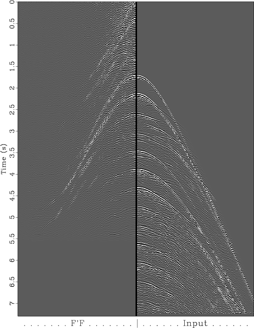
The data and its autocorrelation are in Figure 1.
.
The data and its autocorrelation are in Figure 1.
The autocorrelation ![]() of
of ![]() is
the inverse 2-D Fourier Transform of
is
the inverse 2-D Fourier Transform of
![]() .
Autocorrelations
.
Autocorrelations ![]() satisfy the symmetry relation
satisfy the symmetry relation
![]() .
Figure 2
shows only the interesting quadrant of the two independent quadrants.
We see the autocorrelation of a 2-D function has some
resemblance to the function itself but differs in important ways.
.
Figure 2
shows only the interesting quadrant of the two independent quadrants.
We see the autocorrelation of a 2-D function has some
resemblance to the function itself but differs in important ways.
Instead of messing with two different functions ![]() and
and ![]() to divide,
let us divide
to divide,
let us divide ![]() by itself.
This sounds like
by itself.
This sounds like ![]() but we will
watch what happens when we do the division carefully
avoiding zero division in the ways we usually do.
but we will
watch what happens when we do the division carefully
avoiding zero division in the ways we usually do.
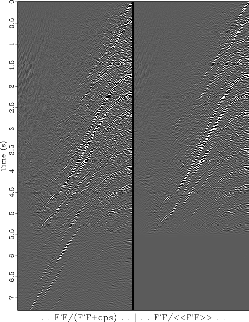
Figure 2 shows
what happens with
|
|---|
|
antoine10
Figure 1. 2-D data (right) and a quadrant of its autocorrelation (left). Notice the longest nonzero time lag on the data is about 5.5 sec which is the latest nonzero signal on the autocorrelation. |
|
|
|
|---|
|
antoine11
Figure 2. Equation 7 (left) and equation 8 (right). Both ways of dividing by zero give similar results. |
|
|
|
|
|
|
Model fitting by least squares |