Model fitting by least squares

FLATTENING 3-D SEISMIC DATA

Here is an expression that on first sight seems to say nothing:

$$\nabla \tau \eq \left[ \begin{array}{c} \frac{\partial \tau... ...} \\ \\ \frac{\partial \tau}{\partial y} \end{array}\right]$$ (82)

Equation (82) looks like a tautology, a restatement of basic mathematical notation. But it is a tautology only if $\tau (x , y )$ is known and the derivatives come from it. When $\tau (x , y )$ is not known but the partial derivatives are observed, then, we have two measurements at each $(x , y )$ location for the one unknown $\tau$ at that location. In Figure , we have seen how to flatten 2-D seismic data. The 3-D process $(x,y,\tau)$ is much more interesting because of the possibility encountering a vector field that cannot be derived from a scalar field.

The easy case is when you can move around the $(x , y )$ plane adding up $\tau$ by steps of $d\tau/dx$ and $d\tau/dy$ and find upon returning to your starting location that the total time change $\tau$ is zero. When $d\tau/dx$ and $d\tau/dy$ are derived from noisy data, such sums around a path often are not zero. Old time seismologists would say, ``The survey lines don't tie.'' Mathematically, it is like an electric field vector that may be derived from a potential field unless the loop encloses a changing magnetic field.

We would like a solution for $\tau$ that gives the best fit of all the data (the stepouts $d\tau/dx$ and $d\tau/dy$) in a volume. Given a volume of data $d(t , x , y )$, we seek the best $\tau (x , y )$ such that $w(t , x , y )= d (t-\tau (x , y ), x , y )$ is flattened. Let us get it.

We write a regression, a residual ${\bf r}$ that we minimize to find a best fitting $\tau (x , y )$ or maybe $\tau (x , y , t )$. Let $d$ be the measurements in the vector in equation (82), the measurements throughout the $(t , x , y )$-volume. Expressed as a regression, equation (82) becomes:

$${\bf0} \quad \approx\quad {\bf r} \eq \nabla \tau \ -\ {\bf d}$$ (83)

Figure 9 shows slices through a cube of seismic data. A paper book is inadequate to display all the images required to compare before and after (one image of output is blended over multiple images of input), therefore, we move on to a radar application of much the same idea, but in 2-D instead of 3-D.

chev
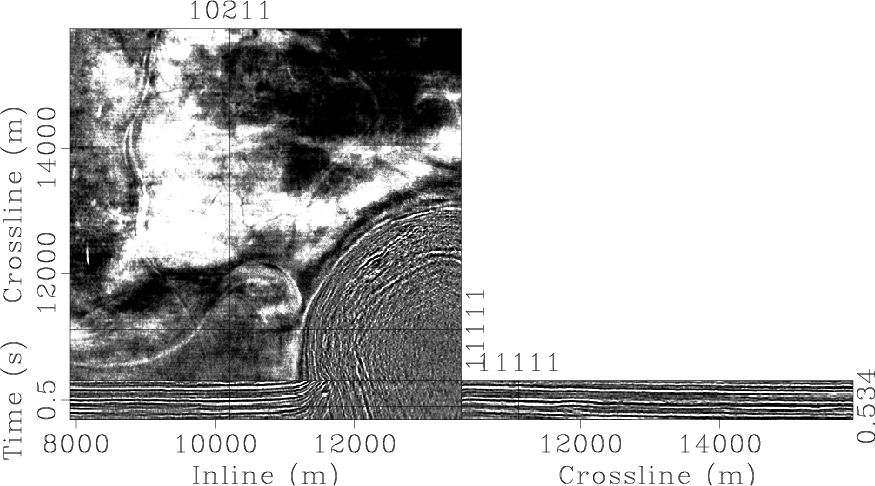
Figure 9. [Jesse Lomask] Chevron data cube from the Gulf of Mexico. Shown are three planes within the cube. A salt dome (lower right corner in the top plane) has pushed upward, dragging bedding planes (seen in the bottom two orthogonal planes) along with it.

Let us see how the coming 3-D illustrations were created. First we need code for vector gradient with its adjoint, negative vector divergence. Here it is: api/c/igrad2.c

    for (i2=0; i2 < n2-1; i2++) {  
	for (i1=0; i1 < n1-1; i1++) {
	    i = i1+i2*n1;
	    if (adj) {
		p[i+1]  += r[i]; 
		p[i+n1] += r[i+n12];
		p[i]    -= (r[i] + r[i+n12]);
	    } else {
		r[i]     += (p[i+1]  - p[i]); 
		r[i+n12] += (p[i+n1] - p[i]);
	    }
	}
    }

In a kind of magic, all we need to fit our regression (82) is to pass the igrad2 module to the Krylov subspace solver, simple solver using cgstep, but first we need to compute d by calculating $dt/dx$ and $dt/dy$ between all the mesh points.

do iy=1,ny { # Calculate x-direction dips: px 
             call puck2d(dat(:,:,iy),coh_x,px,res_x,boxsz,nt,nx) 
           } 
do ix=1,nx { # Calculate y-direction dips: py 
             call puck2d(dat(:,ix,:),coh_y,py,res_y,boxsz,nt,ny) 
           } 
do it=1,nt { # Integrate dips: tau 
             call dipinteg(px(it,:,:),py(it,:,:),tau,niter,verb,nx,ny) 
           }

The code says first to initialize the gradient operator. Convert the 2-D plane of $dt/dx$ to a vector. Likewise $dt/dy$. Concatenate these two vectors into a single column vector d like in equation (82). Tell the simple solver to make its steps with to use cgstep with the linear operator igrad2.

Model fitting by least squares