Model fitting by least squares

INVERSE NMO STACK

To illustrate an example of solving a huge set of simultaneous equations without ever writing down the matrix of coefficients, we consider how back projection can be upgraded toward inversion in the application called moveout and stack.

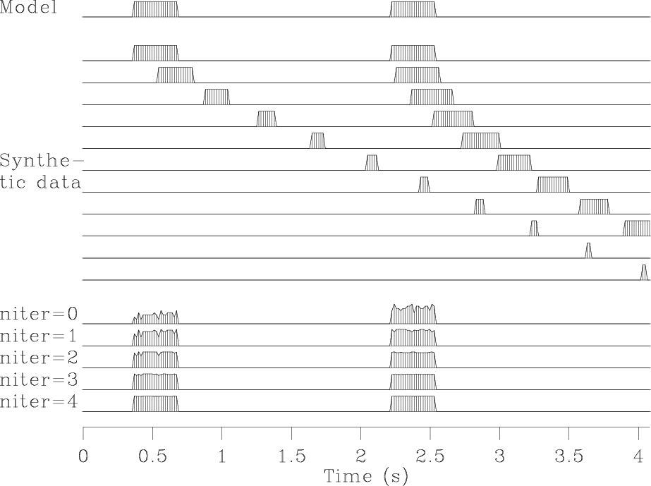
invstack Figure 8. Top is a model trace $\bold m$. Next, are the synthetic data traces, $\bold d = \bold F \bold m$. Then, labeled niter=0 is the stack, a result of processing by adjoint modeling. Increasing values of niter show $\bold m$ as a function of iteration count in the fitting goal $\bold d \approx \bold F \bold m$. (Carlos Cunha-Filho)

The seismograms at the bottom of Figure 8 show the first four iterations of conjugate-direction inversion. You see the original rectangle-shaped waveform returning as the iterations proceed. Notice also on the stack that the early and late events have unequal amplitudes, but after enough iterations match the original model. Mathematically, we can denote the top trace as the model $\bold m$, the synthetic data signals as $\bold d = \bold F \bold m$, and the stack as $\bold F\T\,\bold d$. The conjugate-gradient algorithm optimizes the fitting goal $\bold d \approx\bold F \bold x$ by variation of $\bold x$, and the figure shows $\bold x$ converging to $\bold m$. Because there are 256 unknowns in $\bold m$, it is gratifying to see good convergence occurring after the first four iterations. The fitting is done by module invstack, which is just like cgtest except that the matrix-multiplication operator matmult has been replaced by imospray. Studying the program, you can deduce that, except for a scale factor, the output at niter=0 is identical to the stack $\bold M\T \bold d$. All the signals in Figure 8 are intrinsically the same scale.

user/gee/invstack.c

void invstack(int nt, float *model, int nx, const float *gather, 
	      float t0, float x0, 
	      float dt, float dx, float slow, int niter) 
/*< NMO stack by inverse of forward modeling */
{
    imospray_init( slow, x0,dx, t0,dt, nt, nx);
    sf_tinysolver( imospray_lop, sf_cgstep, 
		   nt, nt*nx, model, NULL, gather, niter);
    sf_cgstep_close ();  
    imospray_close ();  /* garbage collection */
}

This simple inversion is inexpensive. Has anything been gained over conventional stack? First, though we used nearest-neighbor interpolation, we managed to preserve the spectrum of the input, apparently all the way to the Nyquist frequency. Second, we preserved the true amplitude scale without ever bothering to think about (1) dividing by the number of contributing traces, (2) the amplitude effect of NMO stretch, or (3) event truncation.

With depth-dependent velocity, wave fields become much more complex at wide offset. NMO soon fails, but wave-equation forward modeling offers interesting opportunities for inversion.

Model fitting by least squares