|
|
|
|
Regularization is model styling |
|
|---|
|
wellseis
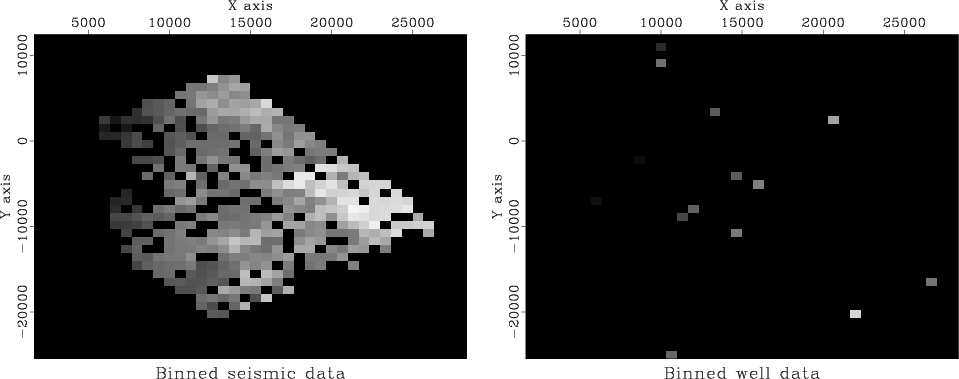
Figure 6. Binning by data push. Left is seismic data. Right is well locations. Values in bins are divided by numbers in bins. (Toldi) |
|
|
|
|---|
|
misseis
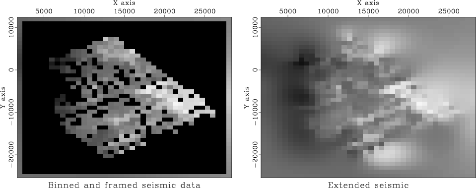
Figure 7. Seismic binned (left) and extended (right) by minimizing energy in |
|
|
There are basically two ways to handle boundary conditions. First, as we did in Figure 1, by using a transient filter operator that assumes zero outside to the region of interest. Second is to use an internal filter operator. Internal filters introduce the hazard that solutions could be growing at the boundaries. Growing solutions are rarely desirable. In that case, it is better to assign boundary values, which is what I did here in Figure 7. I did not do it because it is better, but did it to minimize the area surrounding the data of interest.
The first job is to fill the gaps in the seismic data.
We did such a job in one dimension in Figures 1-5.
More computational details later come later.
Let us call the extended seismic data ![]() .
.
Think of a map of a model space ![]() of infinitely many hypothetical wells that must match the real wells,
where we have real wells.
We must find a map that matches the wells exactly
and somehow matches the seismic information elsewhere.
Let us define the vector
of infinitely many hypothetical wells that must match the real wells,
where we have real wells.
We must find a map that matches the wells exactly
and somehow matches the seismic information elsewhere.
Let us define the vector ![]() , as shown in Figure 6
so
, as shown in Figure 6
so ![]() is
observed values at wells and zeros elsewhere.
is
observed values at wells and zeros elsewhere.
Where the seismic data contains sharp bumps or streaks,
we want our final Earth model to have those features.
The wells cannot provide the rough features, because the wells
are too far apart to provide high-spatial frequencies.
The well information generally conflicts with the seismic data
at low-spatial frequencies because of systematic discrepancies between
the two types of measurements.
Thus we must accept that ![]() and
and ![]() may differ
at low-spatial frequencies (where gradient and Laplacian are small).
may differ
at low-spatial frequencies (where gradient and Laplacian are small).
Our final map ![]() would be very unconvincing if
it simply jumped from a well value at one point
to a seismic value at a neighboring point.
The map would contain discontinuities around each well.
Our philosophy of finding an Earth model
would be very unconvincing if
it simply jumped from a well value at one point
to a seismic value at a neighboring point.
The map would contain discontinuities around each well.
Our philosophy of finding an Earth model ![]() is that our Earth map should contain no obvious
``footprint'' of the data acquisition (well locations).
We adopt the philosophy that the difference
between the final map (extended wells),
and the seismic information
is that our Earth map should contain no obvious
``footprint'' of the data acquisition (well locations).
We adopt the philosophy that the difference
between the final map (extended wells),
and the seismic information
![]() should be smooth.
Thus,
we seek the minimum residual
should be smooth.
Thus,
we seek the minimum residual ![]() ,
which is the roughened difference between the seismic data
,
which is the roughened difference between the seismic data ![]() and the map
and the map ![]() of hypothetical omnipresent wells.
With roughening operator
of hypothetical omnipresent wells.
With roughening operator ![]() we fit:
we fit:
| (13) |
Now, we prepare some roughening operators ![]() .
We have already coded a 2-D gradient operator
igrad2.
Let us combine it with its adjoint to get the 2-D Laplacian operator.
(You might notice that the Laplacian operator is ``self-adjoint,'' meaning
that the operator does the same calculation that its adjoint does.
Any operator of the form
.
We have already coded a 2-D gradient operator
igrad2.
Let us combine it with its adjoint to get the 2-D Laplacian operator.
(You might notice that the Laplacian operator is ``self-adjoint,'' meaning
that the operator does the same calculation that its adjoint does.
Any operator of the form
![]() is self-adjoint because
is self-adjoint because
![]() . )
. )
    for     (i2=0; i2 < n2; i2++) {
	for (i1=0; i1 < n1; i1++) {
	    j = i1+i2*n1;

	    if (i1 > 0) {
		if (adj) {
		    p[j-1] -= r[j];
		    p[j]   += r[j];
		} else {
		    r[j] += p[j] - p[j-1];
		}
	    }
	    if (i1 < n1-1) {
		if (adj) {
		    p[j+1] -= r[j];
		    p[j]   += r[j];
		} else {
		    r[j] += p[j] - p[j+1];
		}
	    }

	    if (i2 > 0) {
		if (adj) {
		    p[j-n1] -= r[j];
		    p[j]    += r[j];
		} else {
		    r[j] += p[j] - p[j-n1];
		}
	    }
	    if (i2 < n2-1) {
		if (adj) {
		    p[j+n1] -= r[j];
		    p[j]    += r[j];
		} else {
		    r[j] += p[j] - p[j+n1];
		}
	    }
	}
    }
|
void lapfill(int niter   /* number of iterations */,
	     float* mm   /* model [m1*m2] */,
	     bool *known /* mask for known data [m1*m2] */)
/*< interpolate >*/
{
    if (grad) {
	sf_solver (sf_igrad2_lop, sf_cgstep, n12, 2*n12, mm, zero,
		   niter, "x0", mm, "known", known,
		   "verb", verb, "end");
    } else {
	sf_solver (laplac2_lop, sf_cgstep, n12, n12, mm, zero,
		   niter, "x0", mm, "known", known,
		   "verb", verb, "end");
    }
    sf_cgstep_close ();
}
|
Subroutine lapfill()
can be used for each of our two applications:
(1) extending the seismic data to fill space, and
(2) fitting the map exactly to the wells and approximately to the seismic data.
When extending the seismic data,
the initially non-zero components
![]() are fixed
and cannot be changed.
are fixed
and cannot be changed.
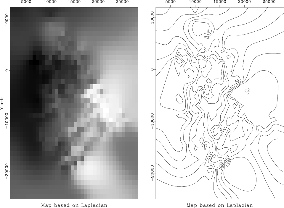
The final map is shown in Figure 8.
|
|---|
|
finalmap
Figure 8. Final map based on Laplacian roughening. |
|
|
Results can be computed with various filters.
I tried both ![]() and
and ![]() .
There are disadvantages of each,
.
There are disadvantages of each,
![]() being too cautious and
being too cautious and
![]() perhaps being too aggressive.
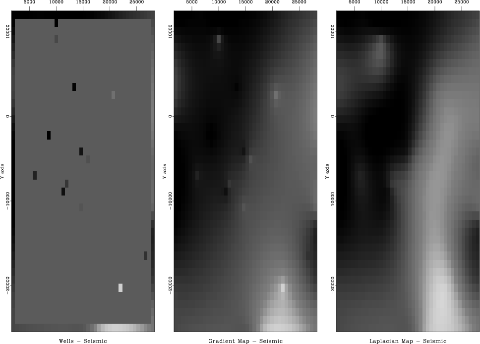
Figure 9 shows the difference
perhaps being too aggressive.
Figure 9 shows the difference ![]() between
the extended seismic data and the extended wells.
Notice that for
between
the extended seismic data and the extended wells.
Notice that for ![]() the difference shows
a localized ``tent pole'' disturbance about each well.
For
the difference shows
a localized ``tent pole'' disturbance about each well.
For ![]() , there could be a large overshoot between wells,
especially if two nearby wells have significantly different values.
I do not see that problem here.
, there could be a large overshoot between wells,
especially if two nearby wells have significantly different values.
I do not see that problem here.
My overall opinion is that the Laplacian does the better job in this case. I have that opinion because in viewing the extended gradient, I can clearly see where the wells are. The wells are where we have acquired data. We would like our map of the world to not show where we acquired data. Perhaps our estimated map of the world cannot help but show where we have and have not acquired data, but we would like to minimize that aspect.
| A good image of the Earth hides our data acquisition footprint. |
|
|---|
|
diffdiff
Figure 9. Difference between wells (the final map) and the extended seismic data. Left is plotted at the wells (with gray background for zero). Center is based on gradient roughening and shows tent-pole-like residuals at wells. Right is based on Laplacian roughening. |
|
|
To understand the behavior theoretically,
recall that in one dimension
the filter ![]() interpolates with straight lines
and
interpolates with straight lines
and ![]() interpolates with cubics.
The reason is that the fitting goal
interpolates with cubics.
The reason is that the fitting goal
![]() ,
leads to
,
leads to
![]() or
or
![]() ; whereas, the fitting goal
; whereas, the fitting goal
![]() leads to
leads to
![]() ,
which is satisfied by cubics.
In two dimensions, minimizing the output of
,
which is satisfied by cubics.
In two dimensions, minimizing the output of ![]() gives us solutions of Laplace's equation with sources at the known data.
It is as if
gives us solutions of Laplace's equation with sources at the known data.
It is as if ![]() stretches a rubber sheet over poles at each well;
whereas,
stretches a rubber sheet over poles at each well;
whereas, ![]() bends a stiff plate.
bends a stiff plate.
Just because ![]() gives smoother maps than
gives smoother maps than ![]() does not mean those maps are closer to reality.
An objectively better choice for the model styling goal is addressed in Chapter
does not mean those maps are closer to reality.
An objectively better choice for the model styling goal is addressed in Chapter ![]() .
It is the same issue we noticed when comparing
Figures 1-5.
.
It is the same issue we noticed when comparing
Figures 1-5.
|
|
|
|
Regularization is model styling |