|
|
|
|
Sigsbee2 Models |
A SConsctuct script found at sigsbee/data2B/fs/ is presented in Table 8. This script translates the segy source data file and converts it into rsf format.
 #########################
 # Sigsbee 2B Shot Data  #
 #########################
from rsf.proj import *

#---- Define Variables and Filenames ---#
data = 'sigsbee2b_nfs.segy'

#------- Import Data ----------#
#- Uses ftp program Fetch
Fetch(data ,'sigsbee')

#-----  Convert Data ----------#
Flow('zdata tzdata ./dhead ./bdhead',data,
     '''
     segyread
     tape=$SOURCE
     tfile=${TARGETS[1]}
     hfile=${TARGETS[2]}
     bfile=${TARGETS[3]}
     ''',stdin=0)

# create sraw(t,o,s): o=full offset, s=shot position, t=time

Flow('ss','tzdata','dd type=float | headermath output="10925+fldr*150" | window')
Flow('oo','tzdata','dd type=float | headermath output="offset"         | window')
Flow('si','ss','math output=input/150')
Flow('oi','oo','math output=input/75')
Flow('os','oi si','cat axis=2 space=n ${SOURCES[1]} | transp | dd type=int')
Flow('sraw','zdata os',
     '''
     intbin head=${SOURCES[1]} xkey=0 ykey=1
     ''')
Flow('shotNfs2B','sraw',
     '''
     put
                           label1=Time       unit1=s
        d2=.02286 o3=0     label2=Offset     unit2=km
        d3=.04572 o3=3.330 label3=Shot-coord unit3=km |
     mutter half=false t0=1.0 v0=6000
     ''')

#-------- Plot Data --------#
Result('zero2Bnfs','shotNfs2B','''window $SOURCE min2=0 max2=0 size2=1
    | grey  pclip=98 color=I screenratio=1.5 gainpanel=a
    label2=Position label1=Time title= label3=  unit2=km unit1=s
    labelsz=3''')

Result('shot702Bnfs','shotNfs2B','''window $SOURCE n3=1 f3=70 |
    grey  pclip=99 color=I gainpanel=a wantframenum=y  unit1=s label1=Time
    label2=Offset unit2=km label3=Shot unit3=km title=
    screenratio=1.35 labelsz=3''')

End()
|
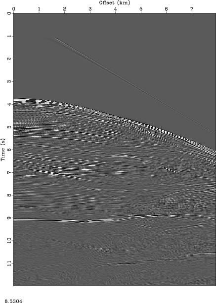
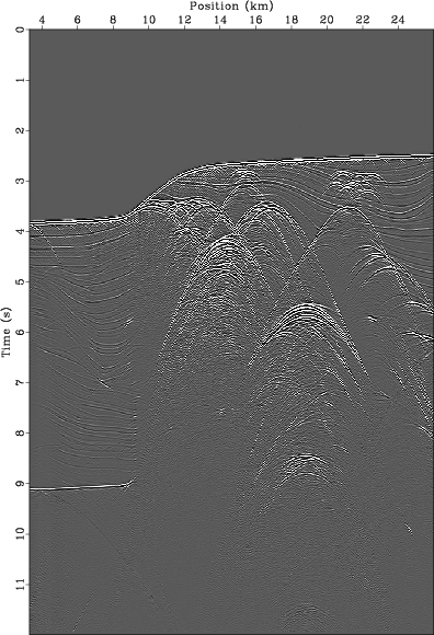
Similar plots are produced for this model. Figure 7 shows an image of shot number 70 taken at 6.5 km into the model. Figure 8 displays the zero offset data acquired on this model.
|
|---|
|
shot702Bnfs
Figure 7. Shot 70 performed in Sigsbee 2B NFS model. |
|
|
|
|---|
|
zero2Bnfs
Figure 8. Sigsbee 2B reflecting surface zero offset data, notice the decreased multiples from the free surface model |
|
|
|
|
|
|
Sigsbee2 Models |