|
|
|
|
Sigsbee2 Models |
For the purposes of this example a shot will be fired at 10 km along the horizontal coordinate and at a depth of 10 meters. Receivers are spread at a depth of 0 meters every 7.62 m (25 ft) along the entire scope of the model. This long receiver cable is impractical but useful for these purposes. Data is recorded on every receiver at time increments of 1 ms 3000 times resulting in 3 seconds of data.
An SConstruct file located within sigsbee/fdmod2A/ properly formats the model and inputs necessary parameters to perform a shot on the Sigsbee model. This file is reproduced below in Table 9.
from rsf.proj import *
import fdmod
##
 # Sigsbee 2A
##
data='sigsbee2a_stratigraphy.sgy'
Fetch(data,'sigsbee')
Flow(['vstr2A','vstr2Ahead'],data,
         '''
         segyread tape=$SOURCE tfile=${TARGETS[1]} |
         put
         o1=0  d1=25     label1=z unit1=ft
         o2=10000 d2=25  label2=x unit2=ft
         ''',stdin=0)
# ------------------------------
par = {
    'nt':7000, 'dt':0.001,'ot':0,    'lt':'t','ut':'s',
    'kt':100,    # wavelet delay
    'nx':3201, 'ox':0, 'dx':0.00762, 'lx':'x','ux':'km',
    'nz':1201, 'oz':0, 'dz':0.00762, 'lz':'z','uz':'km',
    }
# add F-D modeling parameters
fdmod.param(par)
# ------------------------------
# wavelet
Flow('wav',None,
         '''
         spike nsp=1 mag=1 n1=%(nt)d d1=%(dt)g o1=%(ot)g k1=%(kt)d |
         ricker1 frequency=15 |
         scale axis=123 |
         put label1=t label2=x label3=y |
         transp
         ''' % par)
Result('wav',
       'transp | window n1=200 | graph title="" label1="t" label2= unit2=')
# ------------------------------
# experiment setup
Flow('r_',None,'math n1=%(nx)d d1=%(dx)g o1=%(ox)g output=0' % par)
Flow('s_',None,'math n1=1      d1=0      o1=0      output=0' % par)
# receiver positions
Flow('zr','r_','math output="0" ')
Flow('xr','r_','math output="x1"')
Flow('rr',['xr','zr'],
     '''
     cat axis=2 space=n
     ${SOURCES[0]} ${SOURCES[1]} | transp
     ''', stdin=0)
Plot('rr',fdmod.rrplot('',par))
# source positions
Flow('zs','s_','math output=.01')
Flow('xs','s_','math output=10.0')
Flow('rs','s_','math output=1')
Flow('ss',['xs','zs','rs'],
     '''
     cat axis=2 space=n
     ${SOURCES[0]} ${SOURCES[1]} ${SOURCES[2]} | transp
     ''', stdin=0)
Plot('ss',fdmod.ssplot('',par))

# ------------------------------

# Velocity
Flow('vel','vstr2A',
     '''
     scale rscale=.0003048 |
     put o1=%(oz)g d1=%(dz)g  o2=%(oz)g d2=%(dz)g
     ''' % par)

Plot('vel',fdmod.cgrey('''
allpos=y bias=1.5 pclip=100 color=j title=Survey Design labelsz=4 titlesz=6 wheretitle=t
''',par))
Result('vel',['vel','rr','ss'],'Overlay')

# ------------------------------

# density
Flow('den','vel','math output=1')

# ------------------------------
# finite-differences modeling
fdmod.awefd('dat','wfl','wav','vel','den','ss','rr','free=y dens=y',par)

Plot('wfl',fdmod.wgrey('pclip=99 title=Wavefield Movie labelsz=4 titlesz=6 wheretitle=t',par),view=1)

times=['1','2','3','4']
cntr=0
for item in ['9','19','29','39']:
    Result('time'+item,'wfl',
           '''
           window f3=%s n3=1 min1=0 min2=0 | grey gainpanel=a
           pclip=99 wantframenum=y title=Wavefield at %s s labelsz=4
           titlesz=6 screenratio=.375 screenht=2 wheretitle=t
           label1=z label2=x unit1=kft unit2=kft
           ''' % (item,times[cntr]))
    cntr = cntr + 1
Result('dat','window j2=4 j1=2 | transp |' + fdmod.dgrey('pclip=99',par))
End()
|
Typing Command 4 within the sigsbee/fdmod2A/ directory runs the FD modeling script.
This script first constructs the survey acquisition geometry as was previously mentioned. An image of the survey is created and presented in Figure 9.

|
|---|
|
vel
Figure 9. FD model geometry as performed on the Sigsbee 2A velocity model. The X represents the shot while the smaller * symbols represent receivers. The receivers extent along the right hand side although it is not clear in this image. |
|
|
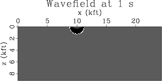
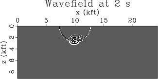
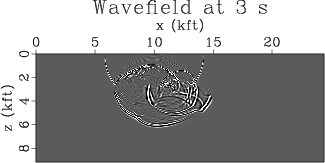
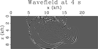
Firing the shot results the propagation of a wavefield which can be seen in the movie wfl.vpl that is generated. Typing Command 5 within the sigsbee/fdmod2A directory displays the wavefield movie.
Four frames from this movie are presented in Figure 10 illustrating the propagation of the wavefield in the model.
|
|---|
|
time9,time19,time29,time39
Figure 10. Images of the propagating wavefield in the Sigsbee model generated by a finite difference model. |
|
|
The resulting data is then presented in the file dat.vpl. This plot is reproduced here in Figure 11.

|
|---|
|
dat
Figure 11. Data gathered by the receivers in the FD model survey. |
|
|
FD models can be performed on the Sigsbee2B model in a similar fashion. The primary change would be in appending line six, the model input file, in the SConstruct file shown in Table 9.
|
|
|
|
Sigsbee2 Models |