Next: Post-stack migration Up: 2-D Seismic Data Processing Previous: Normal moveout (NMO)

Dip moveout (DMO)

In this section, we will apply an improved method of stacking (, ) to the same dataset.

The method starts with generating an ensemble of NMO stacks with constant velocities (Figure 10.)

stacks
Figure 10. Nankai dataset after NMO stacking with an ensemble of constant velocities.

To generate the stacks and display them on your screen, run
```
scons stacks.view
```
Fowler's method works by transforming the stack volume into the frequency-wavenumber $\{\omega,k\}$ domain and applying the velocity mapping according to

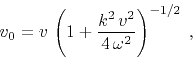$\begin{displaymath} v_0 = \displaystyle v\,\left(1+\frac{k^2\,v^2}{4\,\omega^2}\right)^{-1/2}\;, \end{displaymath}$ (1)

where is NMO stacking velocity (dip-dependent) and is time-migration velocity (dip-independent).
To perform the DMO correction of the constant-velocity stacks (Figure 11), run
```
scons dmo.view
```
Compare the results by running
```
sfpen Fig/dmo.vpl Fig/stacks.vpl
```
Do you notice any improvements?
$\fbox{\parbox{\boxwidth}{\textbf{Answer:} \par }}$

dmo
Figure 11. Nankai dataset after DMO stacking with an ensemble of constant velocities.
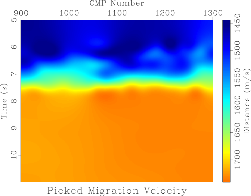
Fowler's method does not generate semblance scans, but it is possible to pick velocities using the power of the stack or the envelope. To pick the DMO-corrected velocity automatically from the envelope (Figure 12), run
```
scons vpick.view
```
vpick
Figure 12. Migration velocity picked automatically from DMO stacks.
After the velocity is picked, we can generate a DMO stack by slicing through the velocity cube. Run
```
scons slice.view
```
to see the result (Figure 13.) To compare results, run
```
sfpen stack.vpl slice.vpl
```
and notice the changes brought by DMO.

slice
Figure 13. (a) DMO stack generated by slicing the constant-velocity stacks.
To evaluate the velocity picking and to observe the change brought by DMO, we can examine a particular CMP location. Run
```
scons envelope.view
```
to display the result (Figure 14.) Modify the SConstruct file to try several other CMP locations and select one that shows the most interesting change.

envelope
Figure 14. Comparison of velocity analysis before and after DMO at a selected CMP location.
Similarly to the previous section, you creative task is to improve the stack (Figure 13) by improving the result of automatic picking. You can use any tools to find a better slice through the velocity cube. Document your work and include the results in this document.
$\fbox{\parbox{\boxwidth}{\textbf{Answer:} %Put your answer here \par }}$