2-D Seismic Data Processing Exercise

Normal moveout (NMO)

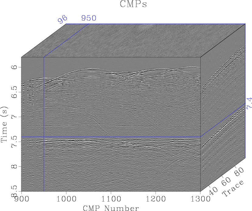
The next step is to apply NMO-based velocity analysis to the Nankai dataset (Keys and Foster, 1998).

1. Run

   scons cmps.view
   

   to display the input data (Figure 4.)

2. What does ``pow pow1=2'' command do?

   Hint: read the documentation for sfpow by running

   sfpow
   

   without arguments or by checking the ``program of the month'' blog post. Modify the pow1= parameter and rerun scons command to observe the change.

   

   cmps
   Figure 4. Nankai dataset after preprocessing and sorting into CMP gathers.

   

   
   

3. We will test our velocity analysis first on one selected CMP gather. Run

   scons cmp1.view
   

   to display the selected gather (Figure 5.)

   

   cmp1
   Figure 5. CMP gather selected for velocity analysis.

   

   
   

4. The process of NMO-based velocity analysis consists of three steps:
   1. Semblance scan.
   2. Picking velocities.
   3. Applying NMO correction.
   The second step is typically done manually and consumes a significant portion of the processor's effort. To speed up the process, we will do it using an automatic picking algorithm.

   Run

   scons vscan.view
   scons nmo.view
   

   to observe the result of velocity analysis on the selected CMP gather using automatic picking (Figure 6.)

   

   vscan,nmo1
   Figure 6. NMO velocity analysis with automatic picking applied to the selected CMP gather.

   

   
   

5. Once we are happy with our picking parameters, we can apply the procedure to the entire 2D line.

   Run

   scons picks.view
   

   to run the semblance analysis with automatic picking on every CMP gather. The result is shown in Figure 7.

   

   picks
   Figure 7. NMO stacking velocity picked automatically from the entire line.

   

   
   

6. Finally, the picked velocity can be applied to NMO and stacking.

   Run

   scons nmos.view
   scons stack.view
   

   to display the result (Figures 8 and 9.)

   

   nmos
   Figure 8. Nankai dataset after normal-moveout correction.

   

   
   

   

   stack
   Figure 9. NMO stack of the Nankai dataset.

   

   
   

7. Your task is to try improving the quality of the stack (Figure 9) by improving the results of automatic picking. To achieve this goal, you can try changing parameters of the picking program sfpick: See http://ahay.org/blog/2012/08/01/program-of-the-month-sfpick/ for more explanation.

2-D Seismic Data Processing Exercise