Time-shift imaging condition for converted waves

Space- and time-shift imaging condition

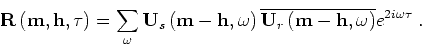
We can formulate a more general imaging condition based on cross-correlation of the source and receiver wavefields after shifting in both time and space. Mathematically, we can represent this process by the relations

$${ \bf u}\left({ \bf m},{ \bf h},t,{\tau}\right) = { \bf u}_s\left({ \bf m}-{ \bf h},t-{\tau}\right) \ast { \bf u}_r\left({ \bf m}+{ \bf h},t+{\tau}\right) \;,$$ (4)

$${ \bf R}\left({ \bf m},{ \bf h},{\tau}\right) = { \bf u}\left({ \bf m},{ \bf h},{\tau},t=0 \right) \;.$$ (5)

Here, ${ \bf h}= \left[ h_x,h_y,h_z \right]$ is a vector describing the local source-receiver separation in the image space, and ${\tau}$ is a time-shift between the source and receiver wavefields prior to imaging. In this imaging condition we do not assume that the source and receiver wavefields maximize image strength at the zero-lag of the space-time cross-correlation. Instead, we probe wavefield similitude at other lags using both shifting in space and time.

This imaging condition can be implemented in the Fourier domain using the expression

$${ \bf R}\left({ \bf m},{ \bf h},{\tau}\right) = \sum_\omega ... ...eft({ \bf m}-{ \bf h},\omega \right)} e^{2i\omega {\tau}} \;.$$ (6)

Special cases of this imaging condition correspond to purely space-shift ${\tau}=0$, when the imaging condition reduces to (Sava and Fomel, 2005a)

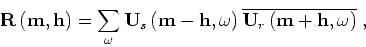$${ \bf R}\left({ \bf m},{ \bf h}\right) = \sum_\omega { \bf... ...verline{{ \bf U}_r\left({ \bf m}+{ \bf h},\omega \right)} \;,$$ (7)

or purely time-shift ${ \bf h}=0$, when the imaging condition reduces to (Sava and Fomel, 2006)

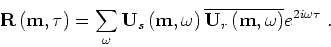$${ \bf R}\left({ \bf m},{\tau}\right) = \sum_\omega { \bf U... ...bf U}_r\left({ \bf m},\omega \right)} e^{2i\omega {\tau}} \;.$$ (8)

The imaging procedures described in this section produce images that can be used for angle decomposition of reflectivity at every image location, thus making this imaging procedure useful for MVA or AVA.

The imaging conditions presented in this section make no assumption on the nature of the source and receiver wavefields We can reconstruct those two wavefields using any type of extrapolation, or using different velocity models for extrapolation of the source and receiver wavefields.

In the following section, we discuss angle-decomposition based on the images obtained by conditions described in the current section. For angle decomposition, we cannot ignore anymore the physical nature of the two wavefields we are comparing, and we need to specify what type of wave (P or S) do the various wavefields correspond to. For the following analysis, we will assume that source wavefields correspond to incident P waves, and receiver wavefields correspond to reflected S waves.

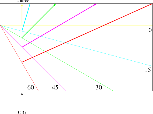
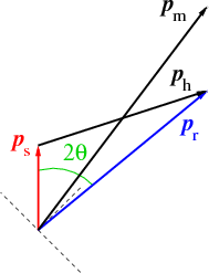
experimentC,vecC
Figure 1. (a) Synthetic PS reflection experiment, and (b) Geometric relations between ray vectors at an image point.

Time-shift imaging condition for converted waves