Time-shift imaging condition for converted waves

Example

We illustrate the imaging and angle-decomposition methods derived in this paper with a synthetic example. The reflectivity model consists of five reflectors of increasing slopes, from $0^\circ$ to $60^\circ$, as illustrated in Figure 1(a). In this experiment, the P-wave velocity is $v_p=3200$ m/s and the S-wave velocity is $v_s=800$ m/s. We chose those velocities in order to capture reflections off the steeper dipping reflectors in a reasonable acquisition geometry. In this experiment, we analyze one common-image gather located at the same horizontal position as the surface seismic source. In this way, the reflector dip is equal to the angle of incidence on each reflector.

Figure 1(a) shows a schematic of a converted-mode (PS) experiment. Given the constant velocity of the model, the single-mode data from the reflector dipping more than $45^\circ$ would not be recorded at the surface. In contrast, the converted-mode data from all reflectors are recorded at the surface.

ps
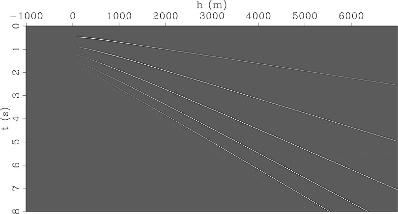
Figure 2. Synthetic PS reflection data

psimg-h
Figure 3. Migrated image for PS data

Figure 2 shows the converted-mode seismic data from all five reflectors. We analyze the positive offsets of the seismic data which contain the reflections from the interfaces in the model.

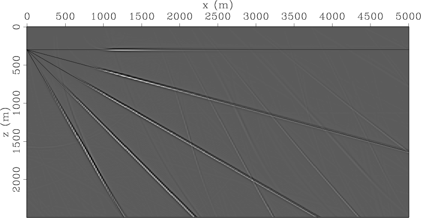
We migrate this shot using one-way wavefield extrapolation using space-shift and time-shift imaging conditions. Figure 3 shows the migrated image at zero shift. As predicted by theory, this image is identical for both space-shift and time-shift imaging conditions when the values of the shift is zero.

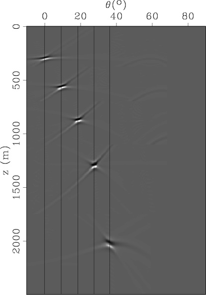
Figures 4(a)-4(c) show different views of the common-image gather (CIG) located at the same horizontal location as the source $x=1000$ m. Panel (a) depicts the CIG resulting from the space-shift imaging condition. The vertical axis represents depth $z$ and the horizontal axis represents horizontal space-shift labeled, for simplicity, $h$. Panel (b) depicts the same CIG after slant-stack in the $z-h$ space. The horizontal axis is the slant-stack parameter, which is related to the reflection angle at every reflector, except for a correction based on dip and the $v_p/v_s$ ratio. Panel (c) depicts the same CIG after transformation to reflection angle $\theta$ using local values of P and S velocities, as well as a correction for the structural dip measured on the migrated image depicted in Figure 3. As expected, each reflector is represented in this final plot at a specific angle of incidence. The vertical lines indicate the correct reflection angles of converted waves reflecting from the interfaces dipping at angles between $0^\circ$ and $60^\circ$.

Figures 5(a)-5(c) show a similar analysis to the one in Figures 4(a)-4(c) but for imaging using time-shift. Panel (a) depicts one CIG at $x=1000$ m, panel (b) depicts the CIG after slant-stack in the $z-{\tau}$ space, and panel (c) depicts the CIG after transformation to reflection angle, including the space-domain corrections for structural dip and $v_p/v_s$ ratio.

As for the space-shift images, the energy corresponding to every reflector from the CIG obtained by time-shift imaging concentrates well in the slant-stack panels, Figures4(b) and 5(b). However, a striking difference occurs in the $z-\theta$ panels: while the energy for every reflector in Figure 4(c) concentrates well, the energy in Figure 5(c) is much less focused, particularly at small angles.

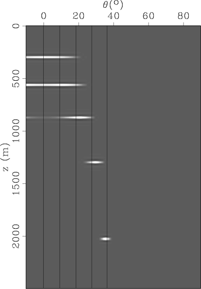
This phenomenon was observed and discussed in detail by Sava and Fomel (2005a), and it is related to the lower angular resolution for time-shift imaging at small angles. This fact is illustrated in Figures 6(a)-6(b) depicting impulse response transformations for time-shift imaging: panel (a) depicts various events in a slant-stack panel, similar to Figure 5(b), and panel (b) depicts the same events in a reflection angle panel, similar to Figure 5(c). At small reflection angles, the angular resolution is low, but it increases at large reflection angles to levels comparable with those of reflections mapped using space-shift imaging. The simple explanation for this phenomenon is that the space-shift transformation involves the $\tan \theta$ trigonometric function whose slope at $\theta \rightarrow 0$ is equal to $1$, while the time-shift transformation involves the $\cos \theta$ function whose slope at $\theta \rightarrow 0$ is equal to $0$. Thus, even given equivalent slant-stack resolutions, the angle resolution around $\theta =0$ is poorer for time-shift imaging than for space-shift imaging because of the different trigonometric function.

psoff-h,psssk-h,psang-h
Figure 4. Common-image gather at $x=1000$ m for space-shift imaging condition: common-image gather (a), slant-stack gather (b) and common-angle gather (c).

psoff-t,psssk-t,psang-t
Figure 5. Common-image gather at $x=1000$ m for time-shift imaging condition: common-image gather (a), slant-stack gather (b) and common-angle gather (c).

ssk,cor
Figure 6. Resolution experiment for time-shift imaging condition: simulated slant-stack (a) and angle-decomposition (b). Although the slant-stack is well focused for all events both function of depth $z$ and slant-stack parameter $\nu$, the resolution of the angle transformation is lower at small angles and higher at large angles.

Time-shift imaging condition for converted waves