|
|
|
|
Imaging overturning reflections by Riemannian Wavefield Extrapolation |
The accuracy of one-way wavefield extrapolation operators maximizes in the direction of extrapolation (vertical for downward continuation; along rays for Riemannian coordinate systems constructed by ray tracing). In addition, for steeply dipping reflectors, the angle of reflection is likely to be relatively small since this reflector is illuminated from a large distance using a small limite acquisition aperture.
It is thus desirable to construct a coordinate system that minimizes the angles between the extrapolation direction, and the directions of wave propagation and normal to the imaged reflectors. One way to achieve this goal is to construct the coordinate system by tracing rays orthogonal to an imaginary line (plane in 3D) located behind the overhanging reflector.
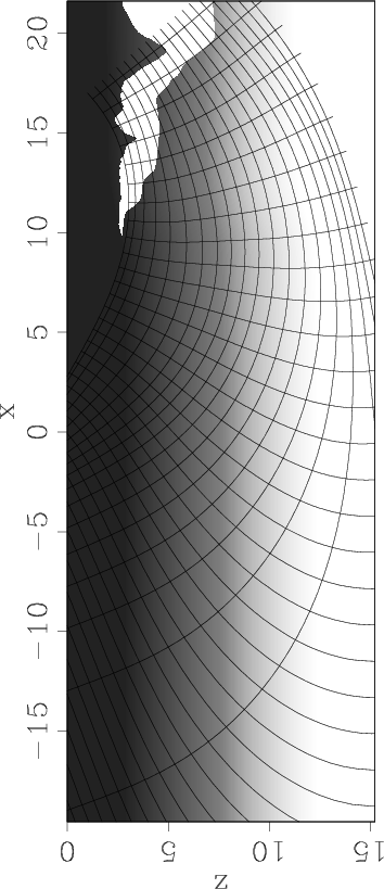
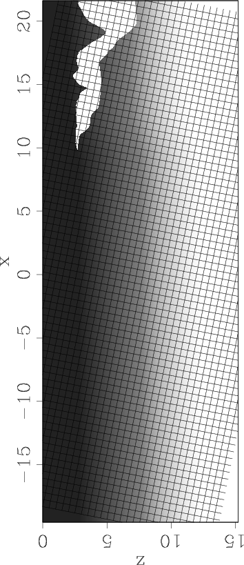
These ideas are illustrated with a model based on the Sigsbee 2A synthetic (Paffenholz et al., 2002) extended vertically and horizontally to allow diving waves from the overhanging salt flank to arrive at the surface. Figure 1(a) shows an example of Riemannian coordinates constructed from ray tracing from behind the salt flank reflector. For comparison, Figure 1(b) shows a Cartesian coordinate system tilted relative to the vertical direction to minimize the angle between the extrapolation direction and the normal to the reflector.
|
|---|
|
cos1,cos2
Figure 1. Riemannian coordinate system (a) and tilted Cartesian coordinate system (b). |
|
|
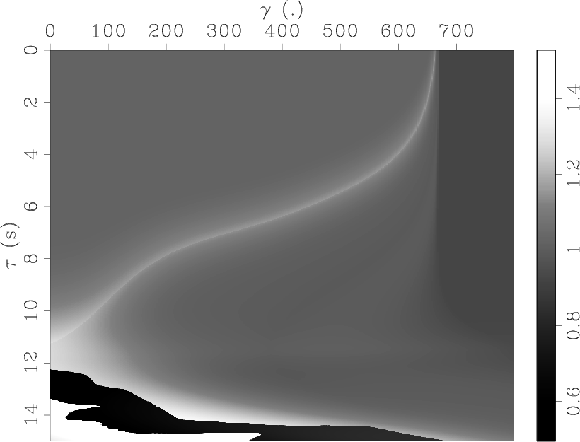
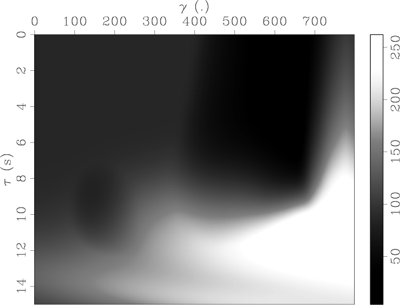
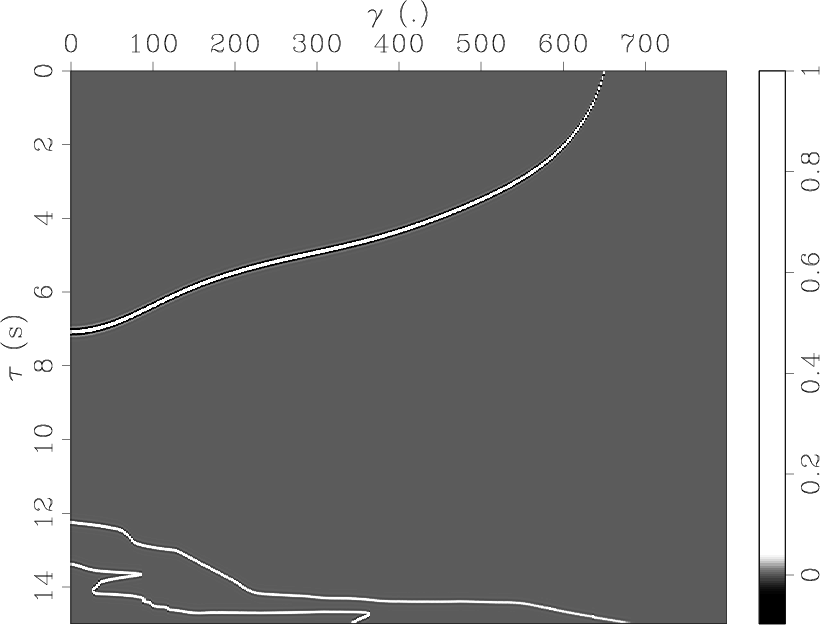
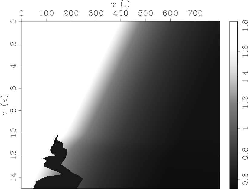
As indicated in the preceding section, we can describe Riemannian coordinate systems with several coefficients incorporating all the information about the coordinate system shape and the extrapolation slowness. For this 2D example, there are two coefficients, ![]() and
and ![]() depicted in Figures 2(a)-2(b) for the Riemannian coordinate system and in Figures 3(a)-3(b) for the tilted Cartesian coordinate system. The plots depict
depicted in Figures 2(a)-2(b) for the Riemannian coordinate system and in Figures 3(a)-3(b) for the tilted Cartesian coordinate system. The plots depict ![]() and
and ![]() function of the Riemannian coordinates,
function of the Riemannian coordinates, ![]() and
and ![]() .
. ![]() has time units and it represents the extrapolation direction, and
has time units and it represents the extrapolation direction, and ![]() is non-dimensional and represents an index of the rays shot from the linear origin behind the imaged reflector.
is non-dimensional and represents an index of the rays shot from the linear origin behind the imaged reflector.
Coefficient ![]() describes the ratio of the extrapolation velocity to the velocity used for ray tracing, and coefficient
describes the ratio of the extrapolation velocity to the velocity used for ray tracing, and coefficient ![]() describes the focusing/defocusing of the coordinate system. In both cases, coefficient
describes the focusing/defocusing of the coordinate system. In both cases, coefficient ![]() since the velocity used for extrapolation is different from the velocity used for the coordinate system. For the Cartesian coordinate system, coefficient
since the velocity used for extrapolation is different from the velocity used for the coordinate system. For the Cartesian coordinate system, coefficient ![]() is a constant, as depicted in Figure 3(b).
is a constant, as depicted in Figure 3(b).
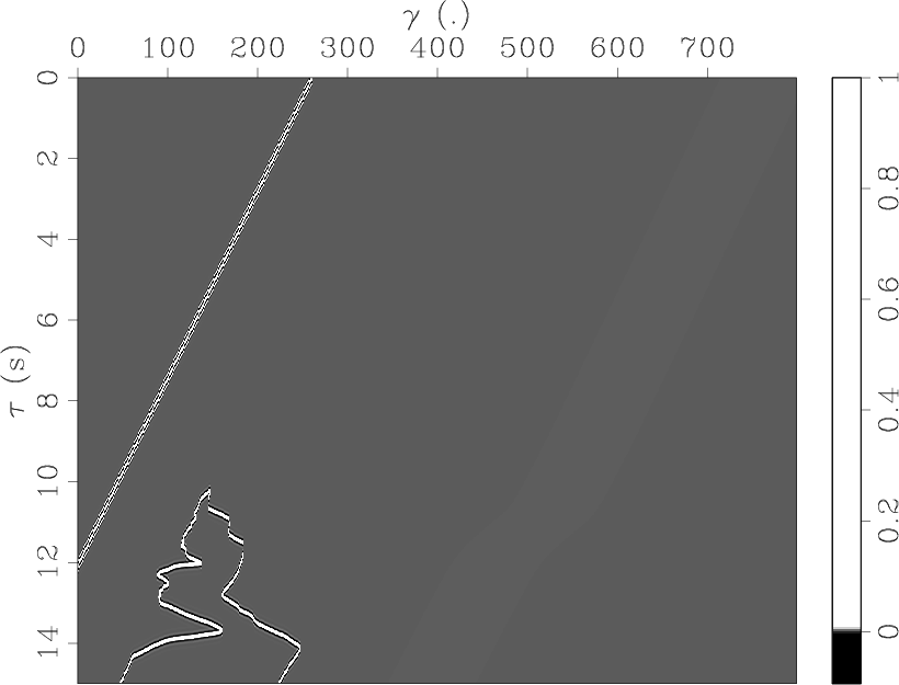
Figures 2(c) and 3(c) depict the acquisition surface and the salt body outline mapped in Riemannian and tilted Cartesian coordinates, respectively. We can observe that in Riemannian coordinates, the overhanging salt flank is nearly orthogonal to the extrapolation direction, unlike its layout in tilted Cartesian coordinates. Therefore, imaging accuracy for such reflectors can be achieved in Riemannian coordinates with lower order extrapolation kernels than in the case of tilted Cartesian coordinates, as demonstrated in the following section.
|
|---|
|
abmRC1a,abmRC1b,edgeRC1
Figure 2. Riemannian coordinate system coefficients, (a) and (b), and outline of acquisition geometry and salt body (c). |
|
|
|
|---|
|
abmRC2a,abmRC2b,edgeRC2
Figure 3. Tilted Cartesian coordinate system coefficients, (a) and (b), and outline of acquisition geometry and salt body (c). |
|
|
|
|
|
|
Imaging overturning reflections by Riemannian Wavefield Extrapolation |