 |
 |
 |
 | Isotropic angle-domain elastic reverse-time migration |  |
![[pdf]](icons/pdf.png) |
Next: Examples
Up: Angle decomposition
Previous: Scalar wavefields
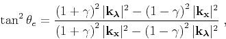
A similar approach can be used for decomposition of the reflectivity
as a function of incidence and reflection angles for elastic
wavefields imaged with extended imaging conditions equations ![[*]](icons/crossref.png) or
. The angle
or
. The angle  characterizing the average angle
between incidence and reflected rays can be computed using the
expression (Sava and Fomel, 2005)
characterizing the average angle
between incidence and reflected rays can be computed using the
expression (Sava and Fomel, 2005)
 |
(12) |
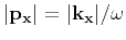
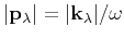
where  is the velocity ratio of the incident and reflected
waves, e.g.
is the velocity ratio of the incident and reflected
waves, e.g.  ratio for incident P mode and reflected S mode.
Figure 1 shows the schematic and the notations used in equation ,
where
ratio for incident P mode and reflected S mode.
Figure 1 shows the schematic and the notations used in equation ,
where
 ,
,
 , and
, and  is the angular
frequency at the imaging location
is the angular
frequency at the imaging location  . The angle decomposition
equation is designed for PS reflections and reduces to
equation for PP reflections when
. The angle decomposition
equation is designed for PS reflections and reduces to
equation for PP reflections when  .
.
Angle decomposition using equation requires computation of
an extended imaging condition with 3D space lags
(
 ), which is computationally costly.
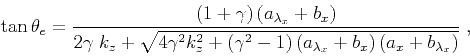
Faster computation can be done if we avoid computing the vertical lag
), which is computationally costly.
Faster computation can be done if we avoid computing the vertical lag
 , in which case the angle decomposition can be done using
the expression (Sava and Fomel, 2005):
, in which case the angle decomposition can be done using
the expression (Sava and Fomel, 2005):
 |
(13) |
where
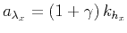 ,
,
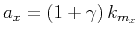 ,
,
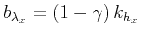 , and
, and
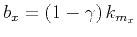 .
Figure 2 shows a model of five reflectors and the extracted angle
gathers for these reflectors at the location of the source. For PP
reflections, they would occur in the angle gather at angles equal with
the reflector slopes. However, for PS reflections, as illustrated in
Figure 2, the reflection angles are smaller than the reflector
slopes, as expected.
.
Figure 2 shows a model of five reflectors and the extracted angle
gathers for these reflectors at the location of the source. For PP
reflections, they would occur in the angle gather at angles equal with
the reflector slopes. However, for PS reflections, as illustrated in
Figure 2, the reflection angles are smaller than the reflector
slopes, as expected.
|
|
|
|
| Isotropic angle-domain elastic reverse-time migration | |
|
Next: Examples
Up: Angle decomposition
Previous: Scalar wavefields
2013-08-29