 |
 |
 |
 | Isotropic angle-domain elastic reverse-time migration |  |
![[pdf]](icons/pdf.png) |
Next: Vector wavefields
Up: Angle decomposition
Previous: Angle decomposition
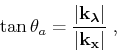
For the case of imaging with the acoustic wave equation, the
reflection angle corresponding to incidence and reflection of P-wave
mode can be constructed after imaging, using mapping based on the
relation (Sava and Fomel, 2005)
 |
(11) |
where  is the incidence angle, and
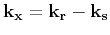 and
and
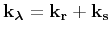 are defined using the source and
receiver wavenumbers,
are defined using the source and
receiver wavenumbers,
 and
and
 . The information
required for decomposition of the reconstructed wavefields as
a function of wavenumbers
. The information
required for decomposition of the reconstructed wavefields as
a function of wavenumbers
 and
and
 is readily
available in the images
is readily
available in the images
 constructed by extended imaging
conditions equations
constructed by extended imaging
conditions equations ![[*]](icons/crossref.png) or .
After angle decomposition, the image
or .
After angle decomposition, the image
 represents a
mapping of the image
from offsets to angles. In other
words, all information for characterizing angle-dependent reflectivity
is already available in the image obtained by the extended imaging
conditions.
represents a
mapping of the image
from offsets to angles. In other
words, all information for characterizing angle-dependent reflectivity
is already available in the image obtained by the extended imaging
conditions.
2013-08-29