next up previous [pdf]

Next: Conclusions Up: Examples Previous: Nankai field data example

Gulf of Mexico field data example

For the final example, we use a Gulf of Mexico field data set (Claerbout, 1995). In this data set, the maximum recording time is 4.0 s with the maximum offset of 3.48 km. The stacked section along with picked migration velocity and Dix velocity is shown in Figure 11. We estimate the initial $w_{dr}(x,z)$ automatically using the method of velocity continuation (Fomel, 2003) followed by 1D Dix inversion to depth which is similar to the workflow for time-to-depth conversion followed by Li and Fomel (2015), and Sripanich and Fomel (2018). Using the Dix velocity, we perform wave-equation time migration as shown in (Figure 12b) which shows improved delineation of faults as compared to the conventional Kirchhoff time migration as shown in (Figure 12a). To convert the migrated section after wave-equation time migration to depth domain, we use fast time to depth conversion algorithm, similarly to the previous example. The inputs to this model are shown in Figure 13. The output of fast time-to-depth algorithm is the grid $t_0-x_0$ Figure 14a which we use to map the wave-equation time migration results from time to depth coordinates (Figure 15a) and the estimated interval velocity in Figure 14b which we use for depth migration in Figure 15b. We compare the final seismic image after time-to-depth conversion process using wave-equation time migration with reverse time migration. The results are comparable to Figure 15b, verifying the effectiveness of the proposed approach.

dstack-gulf vnmo-gulf vinv-gulf
dstack-gulf,vnmo-gulf,vinv-gulf
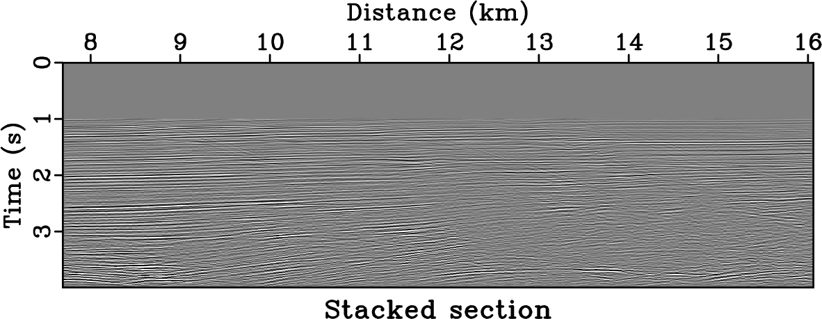
Figure 11.
(a) Stacked section for Gulf of Mexico field data. (b) Time-migration velocity, and (c) Dix velocity.
[pdf] [pdf] [pdf] [png] [png] [png] [scons]

kpstm wetm1f
kpstm,wetm1f
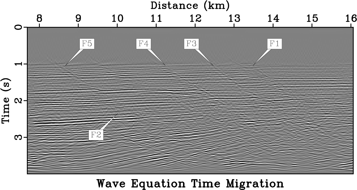
Figure 12.
(a) Image obtained using Kirchhoff time migration , and (b) Image obtained using wave-equation time migration using RTM in image-ray coordinates. Faults marked as F1, F2, F3, F4 and F5 are clearly delineated with the proposed method as compared to the conventional time migration.
[pdf] [pdf] [png] [png] [scons]

refdixgom alphagom betagom
refdixgom,alphagom,betagom
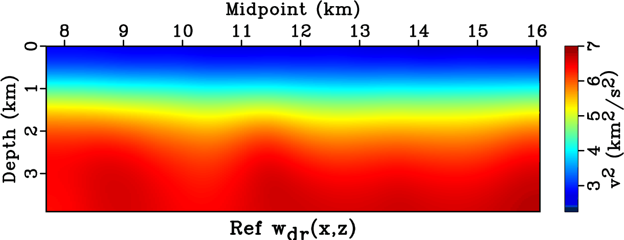
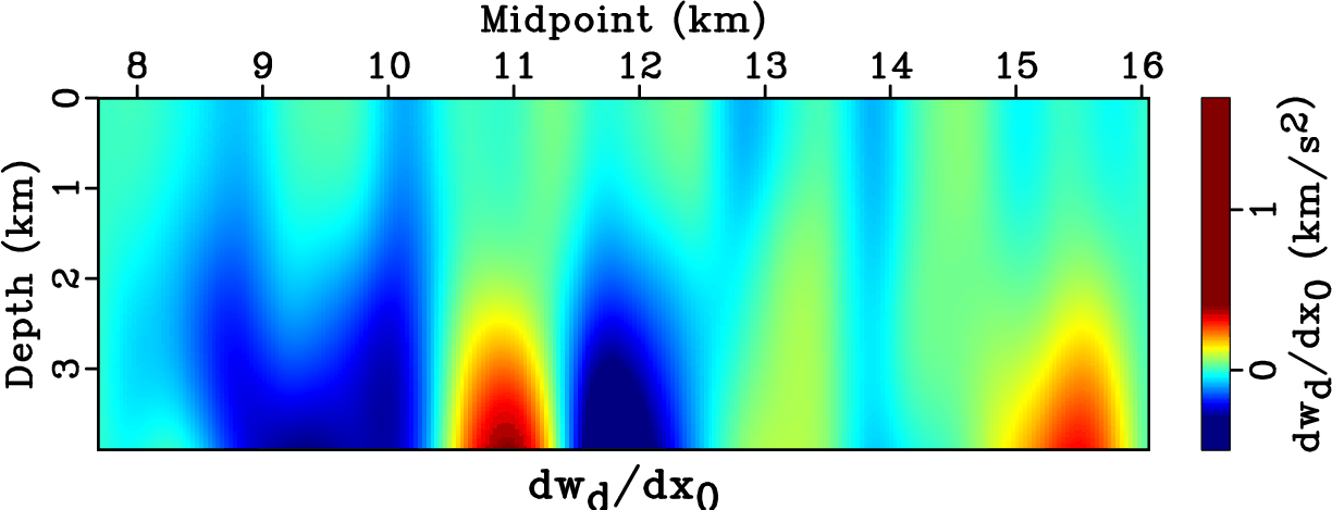
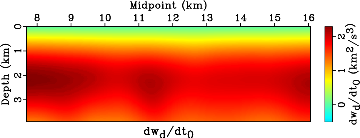
Figure 13.
The inputs for time to depth conversion of velocities for the Gulf of Mexico field data example: Dix velocity squared $w_{dr}$ and its gradients.
[pdf] [pdf] [pdf] [png] [png] [png] [scons]

imagerays finalvgom
imagerays,finalvgom
Figure 14.
(a) Image rays (curves of constant $x_0$) and wavefronts (curves of constant $t_0$). (b) The estimated interval $w(x,z)$ using fast time to depth conversion algorithm for the Nankai field data example.
[pdf] [pdf] [png] [png] [scons]

finalmapdgom rtm
finalmapdgom,rtm
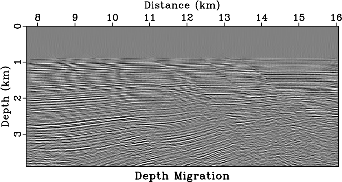
Figure 15.
(a) Image obtained using wave-equation time migration after conversion to Cartesian coordinates. (b) Image obtained using depth migration using RTM in Cartesian coordinates.
[pdf] [pdf] [png] [png] [scons]


next up previous [pdf]

Next: Conclusions Up: Examples Previous: Nankai field data example

2022-05-23