sfiwarp performs mapping between different coordinates.
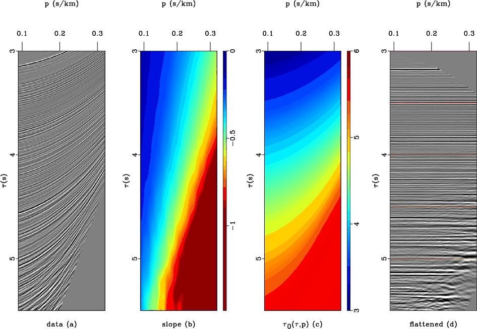
If you have sampled functions $f(x)$ and $y(x)$, sfiwarp with inv=y (the default) finds sampled $f(y)$. If inv=n, sfiwarp takes $f(y)$ and $y(x)$ and finds $f(x)$. In both cases, the sampled $y(x)$ function is supplied in a file specified by warp= parameter. The following example from milano/taupvel/cmp shows a seismic taup-p gather flattening by predictive painting and time warping.
Coordinate mapping is a fundamental data-transformation operation, which finds many applications. The term warping comes from medical imaging. See, for example,
- Wolberg, G., 1990, Digital image warping: IEEE Computer Society Press.
- W. Burnett and S. Fomel, 2009, Moveout analysis by time-warping: 79th Annual International Meeting, SEG, 3710-3714.
The algorithm used in sfiwarp is B-spline interpolation and inverse spline interpolation. If forward warping (inv=n) is $\mathbf{f}_x = \mathbf{B}\,\mathbf{f}_y$, then the inverse transformation (inv=y) is given by the regularized least-squares inverse
$$\mathbf{f}_y = \left(\mathbf{B}^T\,\mathbf{B} + \epsilon^2\,\mathbf{D}\right)^{-1}\,\mathbf{B}^T\,\mathbf{f}_x\;,$$ where $\mathbf{D}$ is the derivative operator. The $\epsilon$ parameter is supplied by eps=. The sampling in $y$ is supplied by n1=, d1=, o1= parameters.
For 2-D and 3-D versions, try sfiwarp2 and sfiwarp3.