|
|
|
|
Deblending of simultaneous-source data using a structure-oriented space-varying median filter |
Next: Including the structure-oriented space-varying Up: Structural-oriented space-varying median filter Previous: Median filter along the
|
|
|
|
Deblending of simultaneous-source data using a structure-oriented space-varying median filter |
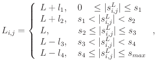
The space-varying median filter can be used in such case where the events are not perfectly flattened. For space-varying median filter, ![]() becomes
becomes ![]() , varying with respect to location
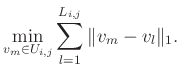
, varying with respect to location ![]() . The new filtering expression is,
. The new filtering expression is,
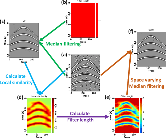
To facilitate an easier understanding of the space-varying median filtering, more specifically the relation among initially filtered data, local similarity, variable filter length, we draw an illustrative picture shown in Figure 5. Figure 5(a) denotes the noisy data. Figure 5(b) shows the map of constant filter length. Figures 5(a) and 5(b) are used to generate the initially filtered data shown in 5(c). Using equation 5, from the original data and the initially filtered data, we can calculate the local similarity map. Utilizing equation 6, we can calculated the map of variable filter length. With the map of variable filter length, we can obtain the finally filtered data shown in Figure 5(f). From this illustration, it is clear that the local similarity clearly detect the main distribution of the useful reflection energy. Those areas with better signal preservation after the initial median filtering are revealed by higher local similarity. The map of variable filter length clearly shows that those noise areas are dealt with very longer filter length while those signal areas correspond to relatively shorter (safer) filter length.
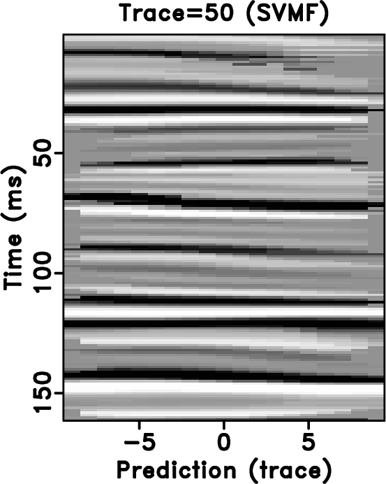
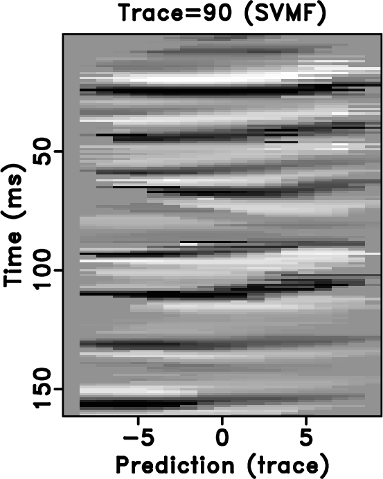
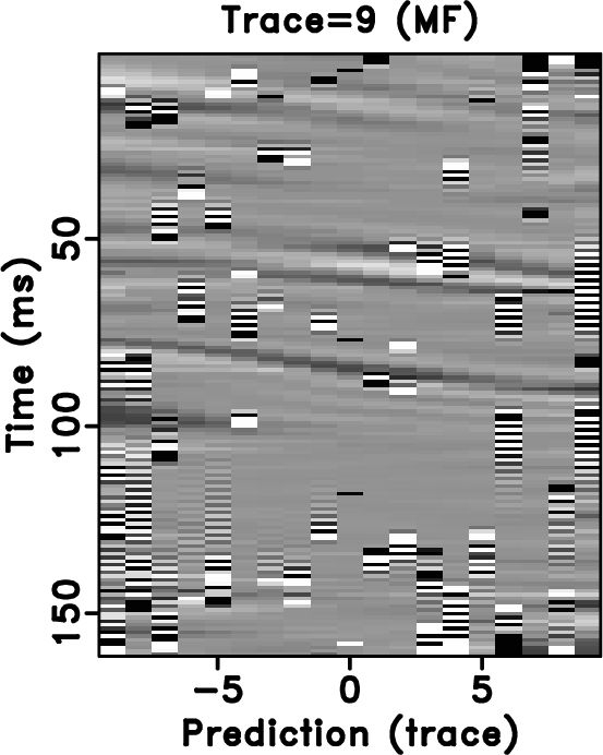
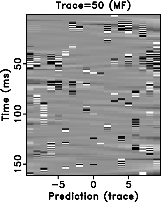
Applying the space-varying median filter in the imperfectly flattened gathers, we can preserve much useful energy that remains curved. Figure 6 shows a comparison between median filter and space-varying median filter in attenuating the spike-like noise when applied to the flattened gathers as shown in Figure 4 from (d) to (f). It is obvious that space-varying median filter helps preserve the energy much better than the median filter. To further confirm this conclusion, we also plot the removed noise sections in Figure 7. It is more salient that the median filter damages more useful energy than the space-varying median filter.

|
|---|
|
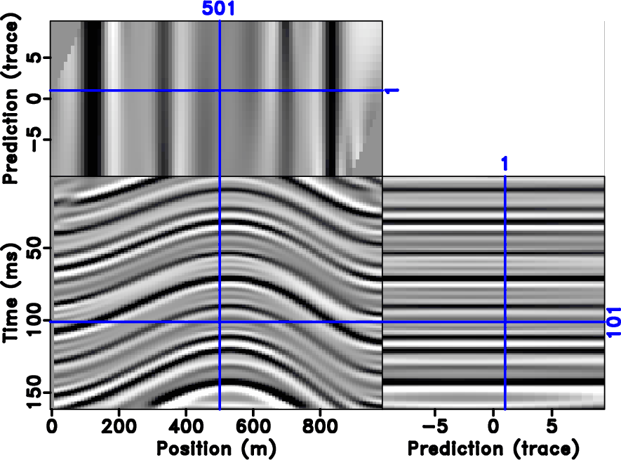
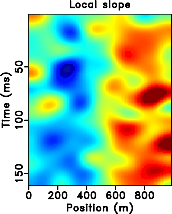
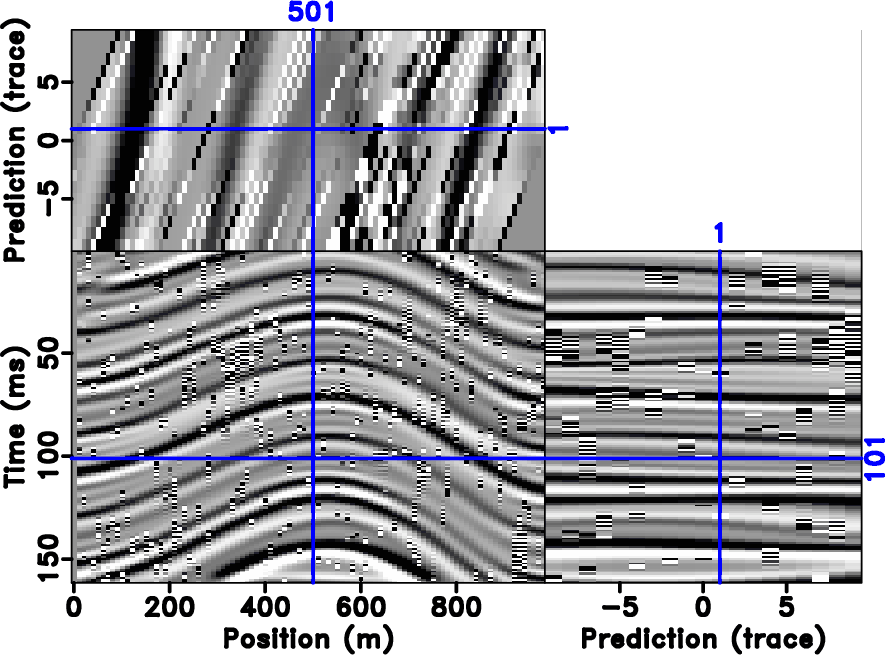
synth,dip,synths-cube,synth-n,dip-n,synths-cuben
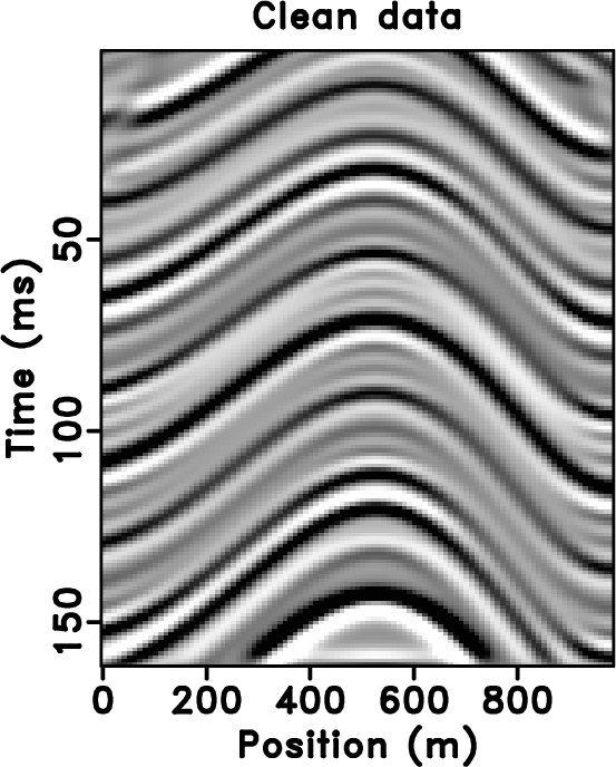
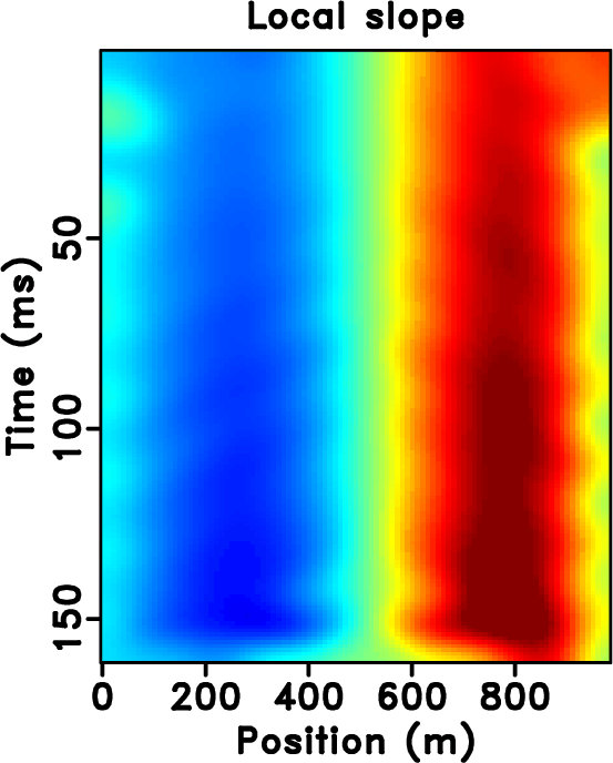
Figure 3. (a) Clean data. (b) Slope estimated from (a). (c) Flattened domain of (a). (d) Noisy data. (e) Slope estimated from (d). (f) Flattened domain of (d). |
|
|
|
|---|
|
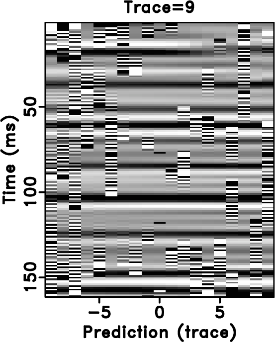
flat1,flat2,flat3,flat1-n,flat2-n,flat3-n
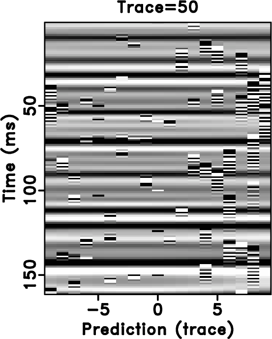
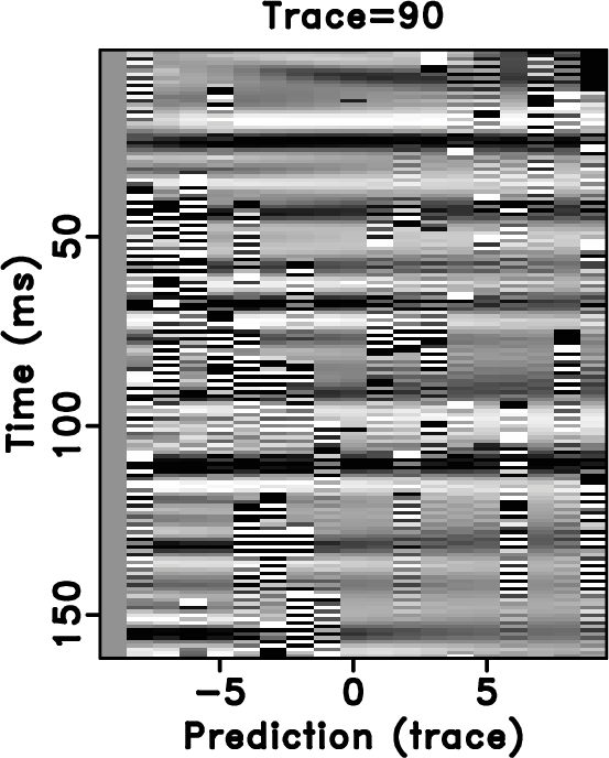
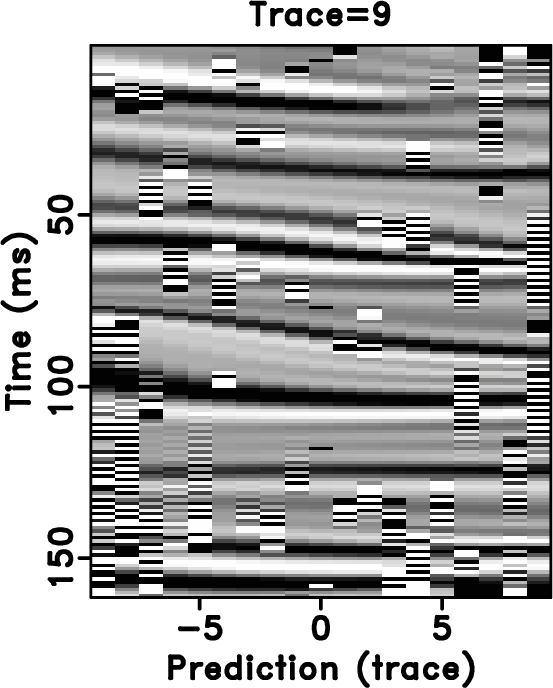
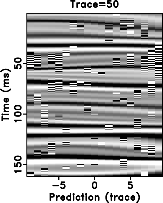
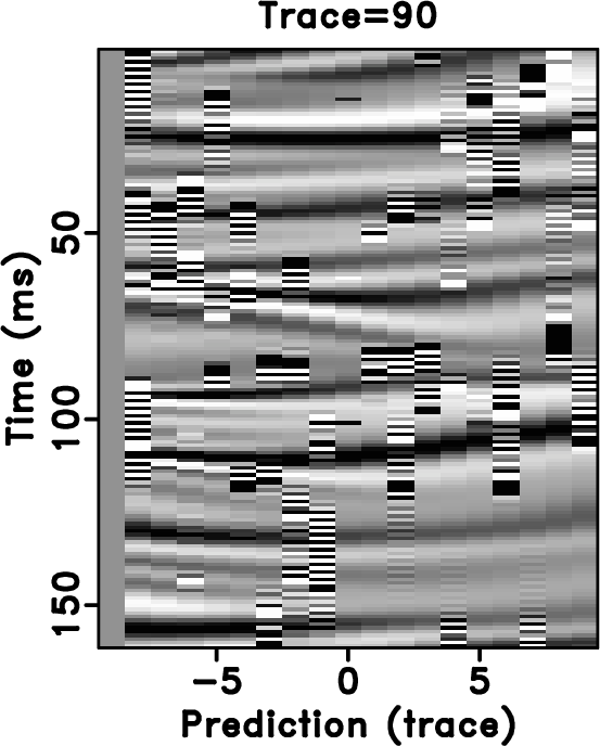
Figure 4. A comparison of “flattened" local windows (predicted dimension) for different space locations. (a)-(c) Flattened gathers for traces 9, 50, 90, using the accurate slope. (d)-(f) “Flattened" gathers for traces 9, 50, 90, using the estimated slope. |
|
|
|
|---|
|
svmf
Figure 5. An illustration of the space-varying median filter. (a) Raw noisy data. (b) A map of constant filter length. (c) Initially filtered data using the constant filter length shown in (b). (d) Calculated local similarity map from (a) and (c) using equation 5. (e) Calculated map of variable filter length using equation 6. (f) Filtered data using the variable filter length shown in (e). |
|
|


|
|---|
|
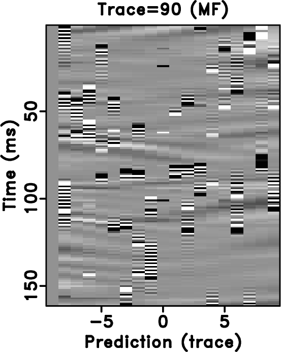
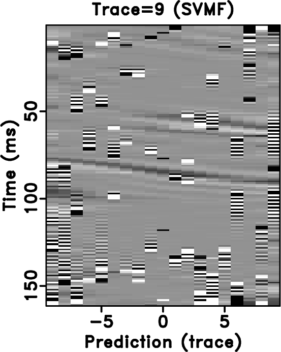
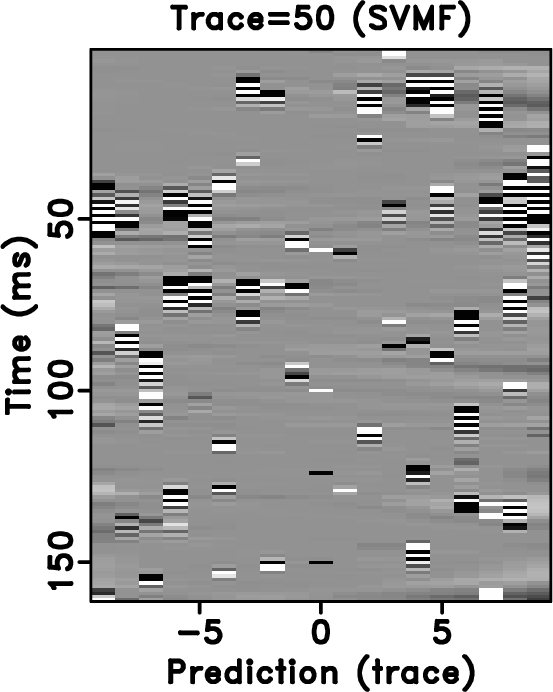
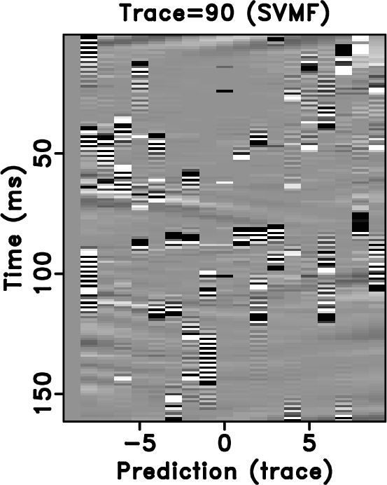
flat1-n-mf,flat2-n-mf,flat3-n-mf,flat1-n-svmf,flat2-n-svmf,flat3-n-svmf
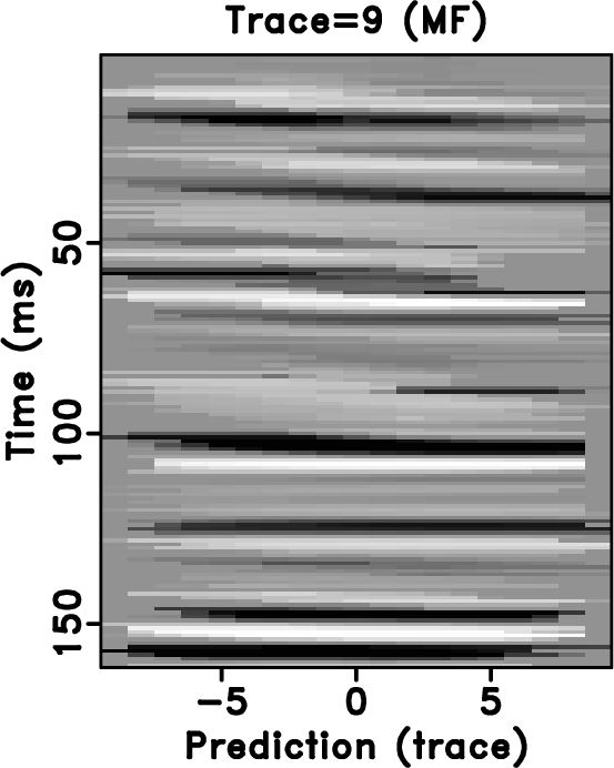
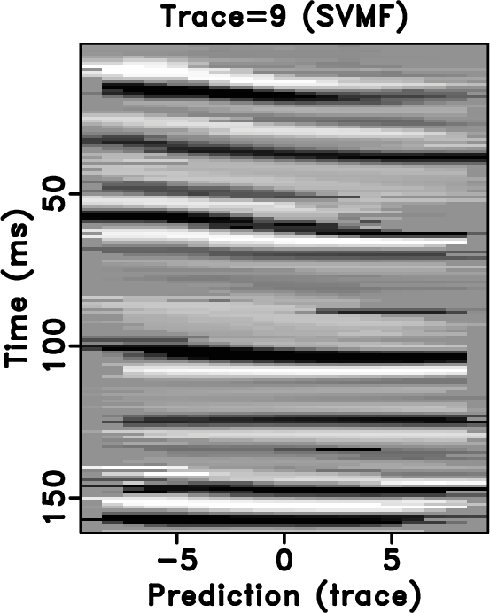
Figure 6. A denoising comparison of “flattened" local windows (predicted dimension) using estimated slope for different space locations. (a)-(c) Denoised gathers for traces 9, 50, 90, using the median filter. (d)-(f) Denoised gathers for traces 9, 50, 90, using the space-varying median filter. Note that although (c) is cleaner, the curving signals are serious damaged. |
|
|
|
|---|
|
flat1-n-mf-dif,flat2-n-mf-dif,flat3-n-mf-dif,flat1-n-svmf-dif,flat2-n-svmf-dif,flat3-n-svmf-dif
Figure 7. A comparison of removed noise. (a)-(c) Removed noise for traces 9, 50, 90, using the median filter. (d)-(f) Removed noise for traces 9, 50, 90, using the space-varying median filter. Note that the median filter removes more coherent energy. |
|
|
|
|
|
|
Deblending of simultaneous-source data using a structure-oriented space-varying median filter |