|
|
|
|
CuQ-RTM: A CUDA-based code package for stable and efficient Q-compensated reverse time migration |
Next: Adaptive stabilization Up: Overview of -RTM Previous: Propagation, compensation, and imaging
|
|
|
|
CuQ-RTM: A CUDA-based code package for stable and efficient Q-compensated reverse time migration |
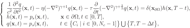
In order to relieve extensive data storage and burdensome disk I/O and thus reach a reasonable compromise between the computer memory requirement and computational complexity, we propose an efficient wavefield reconstruction strategy named CATRC, which combines the efficiency of reverse propagation and the stability of checkpointing. Therefore source wavefields used in imaging condition in equation 4 can be well-reconstructed during time-reversal simulation. Here we denote the reconstructed wavefields as
![]() , which is the solution of
, which is the solution of
It is remarkable that reconstruction by equation 5 is a mathematically stable process, given that the source wavefield is compensated while the reconstructed wavefield from boundary is attenuated. However, this stable reconstruction still suffers from insufficient accuracy due to the fact that we utilize PSM to solve equation 5 with only the recorded forward wavefield at the outermost layer boundary of simulation domain at every time step. This mismatch of simulation accuracy inevitably degrades the performance of the wavefield reconstruction. Fortunately, the time-reversal checkpointing scheme acts as a time-domain regularization that eliminates accumulating errors by replacing the reconstructed wavefield with the stored wavefield at checkpoints (Wang et al., 2017b).
|
|
|
|
CuQ-RTM: A CUDA-based code package for stable and efficient Q-compensated reverse time migration |