Plane-wave orthogonal polynomial transform

We have introduced in detail the theory of plane-wave trace continuation, i.e., how we predict an arbitrary trace in a seismic gather from a random starting trace. We have shown that by discretizing the plane-wave equation. We can derive the spatial trace continuation relation, which can be used for trace prediction. We have presented that during trace continuation, the amplitude of seismic waveforms can be well preserved. Regarding the slope estimation, which is an important factor in the plane-wave trace continuation operator, we introduce the robust slope estimation approach. We also show that the robust slope estimation approach can obtain robust slope estimation in the presence of strong noise. Considering the amplitude-preserving capability of the OPT in a flattened dimension, we can cascade the plane-wave trace continuation operator and the OPT together to obtain a two-folds amplitude-preserving performance during a complete workflow. Thus, we name the cascaded framework as the plane-wave orthogonal polynomial transform. The complete framework for noise attenuation using the plane-wave orthogonal polynomial transform is shown in Algorithm 1.

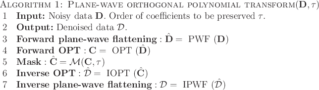
The forward OPT corresponds to inverting $\mathbf{P}^H(\mathbf{P}\mathbf{P}^H)^{-1}$. The inverse OPT corresponds to multiplying the orthogonal polynomial coefficients by $\mathbf{P}$. In algorithm 1, the detailed implementations of the forward plane-wave flattening operator and the inverse plane-wave flattening operator are shown in algorithms 2 and 3, respectively.

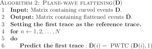
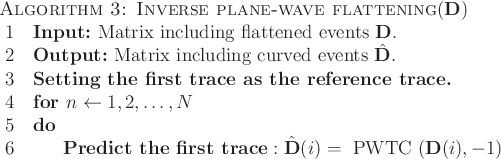
In algorithms 2 and 3, note that $N$ denotes the number of spatial traces. $1$ and $-1$ in the operator PWTC$()$ denote predicting from a trace to the first trace and predicting the first trace to another trace, respectively. $\mathbf{D}(i)$ and $\hat{\mathbf{D}}(i)$ denote the $i$th column (or trace) in the matrix $\mathbf{D}$ and $\hat{\mathbf{D}}$.