In a seismic profile, the amplitude of time  and space
  can be expressed as:
 |
(1) |
where
 is a set of orthogonal polynomials and
  is the number of basis functions and
 is a set of coefficients. The
  is a unit basis function that satisfies the condition:
 |
(2) |
where
 denotes the Kronecker delta. The spectrum defined by
  denotes the energy distribution of the
  domain data in the orthogonal polynomials transform domain. Besides, the low-order coefficients represent the effective energy and the high-order coefficients represent the random noise energy. We provide a detailed introduction about how we construct the orthogonal polynomial basis function in Appendix A.
In a matrix-multiplication form, equation 1 can be expressed as the following equation
 |
(3) |
where
 is constructed from
  ,
,
 is constructed from ,
 is constructed from .
is known and
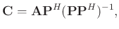
can be constructed using the way introduced in Appendix A. The unknown is
.
can be obtained by inverting the equation 3
is constructed from .
is known and
can be constructed using the way introduced in Appendix A. The unknown is
.
can be obtained by inverting the equation 3
 |
(4) |
where ![$[\cdot]^H$](img27.png) denotes matrix tranpose.
In this paper, we choose
denotes matrix tranpose.
In this paper, we choose  , which indicates that we select 20 orthogonal polynomial basis function to represent the seismic data. Hence, inverting equation
 is simply inverting a
 matrix and is computationally efficient.
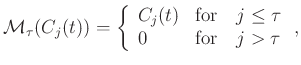
In the OPT method, we need to define the order of coefficients we want to preserve, the process of which corresponds to applying a mask operator to the orthogonal polynomial coefficients. Mask operator can be chosen to preserve low-order coefficients and reject high-order coefficients. It takes the following form:
 |
(5) |
where
 denotes the mask operator, denotes the orthogonal polynomial coefficients at time and order
  .
.
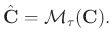
The coefficients after applying the mask operator 5 become
 |
(6) |
The useful signals can be reconstructed by
 |
(7) |
where
 denotes the denoised data.
2020-03-27