|
|
|
|
Five-dimensional seismic data reconstruction using the optimally damped rank-reduction method |
Next: Examples Up: Theory Previous: Optimal weighting for rank
|
|
|
|
Five-dimensional seismic data reconstruction using the optimally damped rank-reduction method |
When the rank is sufficiently large, we assume the estimated signal contains all signal components of the originally observed noisy data and contains less noise than the observed data. To further suppress the residual noise in the estimated signal, we re-analyze
![]() in detail. We can express the newly estimated signal as:
in detail. We can express the newly estimated signal as:
Following Chen et al. (2016c) and Huang et al. (2016),
![]() can be approximated as:
can be approximated as:
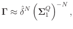
Considering that
![]() ,
,
![]() , and
, and
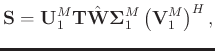
![]() , equation 30 can be expressed as:
, equation 30 can be expressed as:
There are two main advantages of the optimally damped rank reduction method. First, compared with the traditional and damped rank-reduction methods, the optimally damped rank reduction method is insensitive to the rank parameter, making it nearly an adaptive method for rank reduction based seismic denoising and reconstruction. This advantage is important because one of the most troublesome problems in processing complicated seismic data is the selection of the rank. A large rank tends to result in significant residual noise while a small rank tends to damage useful signals. This parameterization problem becomes more seriously when the rank reduction method is applied locally in windows. Because of the insensitivity to rank of the proposed method, one can choose a relatively large rank for all complicated datasets or local patches. Secondly, compared with the optimal weighting based rank reduction method, the proposed method can further suppress the noise components that reside mostly in the smaller singular values. The damping operator is data-driven and can adaptively separate signal and noise in the singular value spectrum further after the optimal weighting.
In the rank-reduction methods, construction of the level-four Hankel matrix is very computationally expensive. Recent advances in the rank reduction based methods show that the construction of the block Hankel matrix is not required. These methods exploit the structure of such matrices to avoid explicitly forming these matrices prior to factorization (Cheng and Sacchi, 2016; Lu et al., 2015). When factorizing data using only 1 or 2 spatial dimensions these approaches are not necessary, but moving to 3 or 4 spatial dimensions is not computationally feasible without considering matrix free approaches. In the current stage, we cannot move from the SVD-based method to SVD-free method because the damping operation has not been derived for the SVD-free case. Although it takes a large computational cost and is not very practically for the time being, it is still a promising algorithm. We will keep on investigating the acceleration of the current algorithm and make it computationally feasible in the future.
|
|
|
|
Five-dimensional seismic data reconstruction using the optimally damped rank-reduction method |
![$\displaystyle \mathbf{Q} = [\mathbf{U}_1^{Q}\quad \mathbf{U}_2^{Q}]\left[\begin...
...egin{array}{c}
(\mathbf{V}_1^{Q})^H\\
(\mathbf{V}_2^{Q})^H
\end{array}\right].$](img84.png)