Construction of the block Hankel matrix for 5-D seismic data

Let $D(t,hx,hy,x,y)$ denote the 5-D seismic data in the time domain, and $D(f,hx,hy,x,y)$ be the data in the frequency domain. For notation convenience, we omit $f$ in the following context and use $D_{k1,k2,k3,k4}$ to denote $D(f,hx,hy,x,y)$. The traditional rank-reduction based methods require the construction of a level-four block Hankel matrix for 5-D seismic data to meet the low-rank assumption. A level-four block Hankel matrix means that we treat a series of level-three block Hankel matrix as elements and arrange them into a Hankel matrix. In a similar way, a level-three block Hankel matrix is constructed from a series of level-two block Hankel matrices while a level-two block Hankel matrix is formed from several standard Hankel matrices.

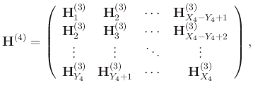
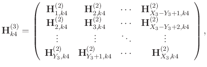
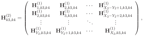
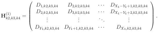
The level-four block Hankel matrix has the following explicit expression:

$$\mathbf{H}^{(4)}=\left(\begin{array}{cccc} \mathbf{H}_{1}^{(3)} &... ...)}&\mathbf{H}_{Y_4+1}^{(3)} &\cdots& \mathbf{H}_{X_4}^{(3)} \end{array}\right),$$ (1)

where

$$\mathbf{H}_{k4}^{(3)}=\left(\begin{array}{cccc} \mathbf{H}_{1,k4}... ...athbf{H}_{Y_3+1,k4}^{(2)} &\cdots&\mathbf{H}_{X_3,k4}^{(2)} \end{array}\right),$$ (2)

and

$$\mathbf{H}_{k3,k4}^{(2)}=\left(\begin{array}{cccc} \mathbf{H}_{1,... ...H}_{Y_2+1,k3,k4}^{(1)} &\cdots&\mathbf{H}_{X_2,k3,k4}^{(1)} \end{array}\right),$$ (3)

and

$$\mathbf{H}_{k2,k3,k4}^{(1)}=\left(\begin{array}{cccc} D_{1,k2,k3,... ..._{Y_1,k2,k3,k4}&D_{Y_1+1,k2,k3,k4} &\cdots&D_{X_1,k2,k3,k4} \end{array}\right).$$ (4)

In order to make all target matrices (from equation 1 to 4) close to square matrices, parameters $Y_i$ are defined as $\lfloor \frac{X_i}{2} \rfloor +1$, $i=1,2,3,4$, where $X_i$ denotes the size of the $i$th dimension. Here, $\lfloor\cdot\rfloor$ denotes the integer part of an input argument.

The process of transforming a four-dimensional hypercube $D_{k1,k2,k3,k4}$ to the block Hankel matrix $\mathbf{H}^{(4)}$ is referred to as the Hankelization process. We can briefly denote this process as:

$$\mathbf{H}^{(4)}=\mathcal{H}D_{k1,k2,k3,k4}.$$ (5)

Another important step in the rank-reduction based method is the rank reduction process, which can be denoted as $\mathcal{F}$.

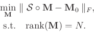
Reconstructing the missing data aims at solving the following equation:

$$\mathcal{S} \circ \mathbf{M} = \mathbf{M}_{0},$$ (6)

where $\mathcal{S}$ is a sampling matrix, $\mathbf{M}=\mathbf{H}^{(4)}$, and $\mathbf{M}_{0}$ denotes the block Hankel matrix with missing entries. $\circ$ denotes element-wise product.

Equation 6 is seriously ill-posed and the low-rank assumption is applied to constrain the model,

$$\begin{split} \min_{\mathbf{M}} &\parallel \mathcal{S} \circ ... ...F, \\ \text{s.t.}&\quad \text{rank}(\mathbf{M})=N. \end{split}$$ (7)

$\parallel \cdot \parallel_F$ denotes the Frobenius norm of an input matrix. The constraint in equation 7 means that we constrain the rank of the block Hankel matrix to be $N$.

The problem expressed in equation 7 can be solved via the following iterative solver:

$$\mathbf{M}_n=a_n \mathbf{M}_{0} + (1-a_n\mathcal{S})\circ \mathcal{F}\mathbf{M}_{n-1},$$ (8)

$a_n$ is an iteration-dependent scalar that linearly decreases from $a_1=1$ to $a_{n_{max}}=0$. $a_n$ is used to alleviate the influence of random noise existing in the observed data.