|
|
|
|
Seismic signal enhancement based on the lowrank methods |
Next: Results Up: Theory Previous: Damped rank-reduction method
|
|
|
|
Seismic signal enhancement based on the lowrank methods |
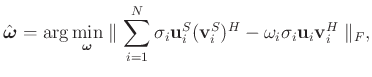
The adaptive weighting operator can be applied to make the traditional rank-reduction method adaptive:
| Symbols | Meanings |
|
|
3D noisy seismic data |
|
|
abbreviated notation of 2D frequency slice |
|
|
|
|
|
block Hankel matrix |
|
|
signal component |
|
|
estimated signal component |
|
|
left singular vector matrix |
|
|
singular-value matrix |
|
|
right singular vector matrix |
|
|
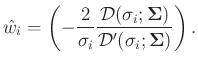
weighting matrix |
|
|
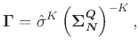
damping matrix |
|
|
damping threshold matrix |
|
|
temporary variable |
|
|
D-transform |
|
|
Hankelization operator |
|
|
thresholding operator |
|
|
averaging operator |
| rank | |
| damping factor |
| Tests | Noisy (dB) | RR (dB) | DRR (dB) | ODRR (dB) |
| Linear synthetic (N=3) | -8.39 | 6.57 | 10.29 | 11.27 |
| Linear synthetic (N=6) | -8.39 | 3.45 | 8.35 | 10.86 |
| Hyperbolic synthetic (N=10) | -2.17 | 8.27 | 9.58 | 9.65 |
| Hyperbolic synthetic (N=20) | -2.17 | 7.04 | 10.08 | 11.00 |
| Tests | FK (s) | RR (s) | DRR (s) | ODRR (s) | ||
| Linear synthetic (N=3) | 0.13 | 2.27 | 2.45 | 2.43 | ||
| Linear synthetic (N=6) | 0.17 | 3.02 | 3.04 | 3.17 | ||
| Hyperbolic synthetic (N=10) | 0.43 | 1.69 | 1.71 | 1.83 | ||
| Hyperbolic synthetic (N=20) | 0.49 | 2.75 | 2.69 | 2.83 |
|
|
|
|
Seismic signal enhancement based on the lowrank methods |
 Tr
Tr![\begin{displaymath}\begin{split}
D'(\sigma;\boldsymbol{\Sigma})&= 2\left[\frac{1...
...athbf{I}-\boldsymbol{\Sigma}^2)^{-2}\right)\right].
\end{split}\end{displaymath}](img78.png)