|
|
|
|
Full waveform inversion and joint migration inversion with an automatic directional total variation constraint |
Next: FWI Example Up: Qu et al.: Directional Previous: Theory of JMI
|
|
|
|
Full waveform inversion and joint migration inversion with an automatic directional total variation constraint |
The extended misfit function with a TV constraint can be expressed as
However, this conventional TV regularization only tends to reduce the horizontal- and vertical-gradients of each gridpoint in the model, regardless of the geological direction of the model. Therefore, TV is not suitable where the local structure has a dominant direction. Unlike general digital images, the spatial changes in the subsurface always follow some specific geological structures, e.g., tilted layers, faults, and edges of a salt body. In this case, we propose FWI/JMI with directional TV and we design the directional TV based on the local dip estimated from a rough reflection image using the plane-wave destruction (PWD) algorithm (Fomel, 2002).
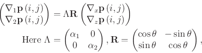
The misfit function with directional TV can be formulated as
Please note that if we assume
![]() and
and
![]() , then
, then ![]() turns into an identity matrix, which means the same weights are put on both directions, and
turns into an identity matrix, which means the same weights are put on both directions, and
![]() also becomes an identity matrix, indicating that the target directions are horizontal and vertical. Therefore, we can see that the conventional TV is actually a special case of the directional TV, and in turn, the directional TV is a more general version of the conventional TV and more suitable to a model with complex geologic structures. In this paper, we solve both FWI/JMI with the conventional TV and FWI/JMI with the directional TV effectively using the split-Bregman iterative algorithm (Goldstein and Osher, 2009). We only show the framework of solving FWI with the directional TV in Algorithm 1, because, as mentioned before, we treat the conventional TV as a special case of directional the TV, and JMI with the conventional TV/directional TV will follow a similar algorithm.
also becomes an identity matrix, indicating that the target directions are horizontal and vertical. Therefore, we can see that the conventional TV is actually a special case of the directional TV, and in turn, the directional TV is a more general version of the conventional TV and more suitable to a model with complex geologic structures. In this paper, we solve both FWI/JMI with the conventional TV and FWI/JMI with the directional TV effectively using the split-Bregman iterative algorithm (Goldstein and Osher, 2009). We only show the framework of solving FWI with the directional TV in Algorithm 1, because, as mentioned before, we treat the conventional TV as a special case of directional the TV, and JMI with the conventional TV/directional TV will follow a similar algorithm.
|
|
|
|
Full waveform inversion and joint migration inversion with an automatic directional total variation constraint |