Seislet-based morphological component analysis using scale-dependent exponential shrinkage

Analysis-based iterative thresholding

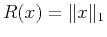
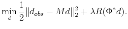
A general inverse problem combined with a priori constraint $R(x)$ can be written as an optimization problem

$$\min_x \frac{1}{2}\Vert d_{obs}-F x\Vert _2^2+\lambda R(x),$$ (1)

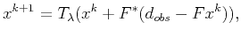
where $x$ is the model to be inverted, and $d_{obs}$ is the observations. To solve the problem with sparsity constraint $R(x)=\Vert x\Vert _1$ , the iterative shrinkage-thresholding (IST) algorithm has been proposed (Daubechies et al., 2004), which can be generally formulated as

$$x^{k+1}=T_{\lambda}(x^{k}+F^*(d_{obs}-Fx^{k})),$$ (2)

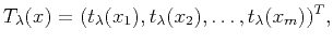
where $k$ denotes the iteration number; and $F^*$ indicates the adjoint of $F$ . $T_{\lambda}(x)$ is an element-wise shrinkage operator with threshold $\lambda$ :

$$T_{\lambda}(x)=(t_{\lambda}(x_1),t_{\lambda}(x_2),\ldots,t_{\lambda}(x_m))^T,$$ (3)

in which the soft thresholding function (Donoho, 1995) is

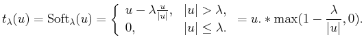$$t_{\lambda}(u)=\mathrm{Soft}_{\lambda}(u)=\left\{\begin{array}{ll... ...rt\leq \lambda. \end{array} \right. =u.*\max(1-\frac{\lambda}{\vert u\vert},0).$$ (4)

Allowing for the missing elements in the data, the observations are connected to the complete data via the relation

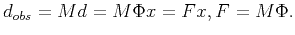$$d_{obs}=Md=M\Phi x=Fx, F=M\Phi.$$ (5)

where $M$ is an acquisition mask indicating the observed and missing values. Assume $\Phi$ is a tight frame such that 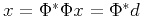$\Phi^*\Phi=\mathrm{Id}$ , $x=\Phi^*\Phi x=\Phi^*d$ . It leads to

$$\begin{array}{ll} d^{k+1} & =\Phi x^{k+1} \\ & =\Phi T_{\lamb... ... =\Phi T_{\lambda}(\Phi^*(d^{k}+(d_{obs}-Md^{k}))), \end{array}$$ (6)

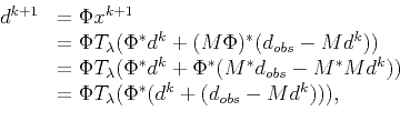
in which we use $M^*=M=(M)^2$ and $Md_{obs}=M^2d=Md$ . Now we define a residual term as $r^{k}=d_{obs}-Md^{k}$ , thus Eq. (6) results in

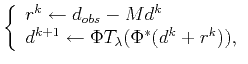$$\left\{ \begin{array}{l} r^{k}\leftarrow d_{obs}-Md^{k} \\ d^{k+1}\leftarrow \Phi T_{\lambda}(\Phi^*(d^{k}+r^{k})), \end{array} \right.$$ (7)

which is equivalent to solving

$$\min\limits_{d}\frac{1}{2}\Vert d_{obs}-Md\Vert _2^2+\lambda R(\Phi^{*}d).$$ (8)

Note that Eq. (8) analyzes the target unknown $d$ directly, without resort to $x$ and $d=\Phi x$ . Eq. (6) is referred to as the analysis formula (Elad et al., 2007). In this paper, we used the analysis formula because it directly addresses the problem in the data domain for the convenience of interpolation and signal separation.

Seislet-based morphological component analysis using scale-dependent exponential shrinkage