Seislet-based morphological component analysis using scale-dependent exponential shrinkage

Trace interpolation

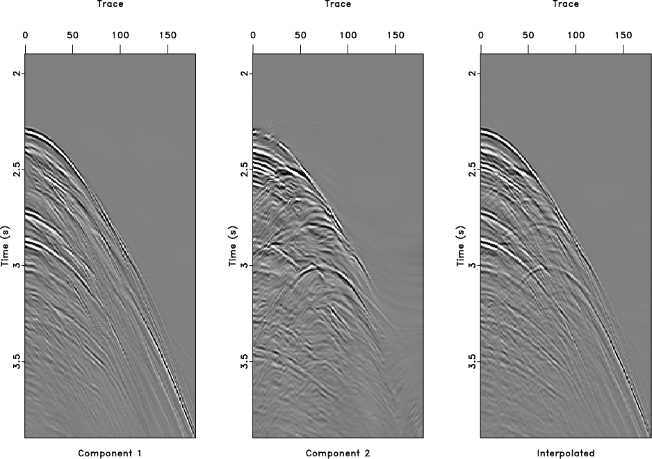
Interpolation of random missing traces is an important task in seismic data processing. Unlike most studies using only one transform, we consider the seismic data having two different components, which can be characterized by a seislet frame composed of seislet transforms associated with two different slopes. PWD filter is utilized to estimate the two dip fields (Fomel, 2002). As shown in Figure 2, the complete data is decimated with a random eliminating rate 25%. 10 iterations are carried out to separate these components. The estimated dips (Figure 3) by PWD indicate that the two separated components exhibit different modes: component 2 has positive and negative dips, corresponding to seismic diffractions, while the events of component 1 are more consistent (most values of the dip are positive). The summation of the two components gives a reasonable interpolation result (right panel of Figure 4.) For comparison, we define the signal-to-noise ratio as $\mathrm{SNR}=10\log_{10}(\frac{\vert s\vert^2}{\vert s-\hat{s}\vert^2})$ to quantify the reconstruction performance. The resulting SNRs using exponential shrinkage, soft, hard, and generalized p-thresholding are 11.98 dB, 11.29 dB, 5.37 dB and 8.94 dB, respectively. It shows that the proposed exponential shrinkage outperforms the existing methods in MCA interpolation. It is important to point out that approximating the $\ell_0$ and $\ell_1$ minimization in a smooth constraint has already been validated in seismic interpolation applications by Cao et al. (2011). The use of exponential shrinkage enriches the sparsity-promoting shaping operator and extends the smooth constraint to MCA approach.

data
Figure 2. The observed seismic data (right) to be interpolated is obtained by 25% random eliminating the complete data (left).

dips
Figure 3. PWD estimated dips: dip estimation for component 1 (Left) are positive-valued, while dip for component 2 includes negative and positive values.

interp
Figure 4. From left to right: MCA reconstructed component 1, component 2 and the final interpolated data.

Seislet-based morphological component analysis using scale-dependent exponential shrinkage