 |
 |
 |
 | RTM using effective boundary saving: A staggered grid GPU implementation |  |
![[pdf]](icons/pdf.png) |
Next: Memory manipulation
Up: GPU implementation using CPML
Previous: GPU implementation using CPML
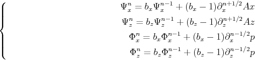
To combine the absorbing effects into the acoustic equation, CPML boundary condition is such a nice way that we merely need to combine two convolutional terms into the above equations:
 |
(13) |
where  ,
,  are the convolutional terms of
  and
and  ;
;  ,
,  are the convolutional terms of
  and
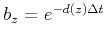
and  . These convolutional terms can be computed via the following relation:
 |
(14) |
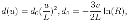
where
 and
and
 . In the absorbing layers, the damping parameter
  we used is (Collino and Tsogka, 2001):
 |
(15) |
where  indicates the PML thickness;
  represent the distance between current position (in PML) and PML inner boundary.
  is always chosen as
 . For more details about the derivation of CPML, the interested readers are referred to Collino and Tsogka (2001) and Komatitsch and Martin (2007). The implementation of CPML boundary condition is easy to carry out: in each iteration the wavefield extrapolation is performed according to the first equation in (13); it follows by adding the convolutional terms in terms of (14).
|
|
|
|
| RTM using effective boundary saving: A staggered grid GPU implementation | |
|
Next: Memory manipulation
Up: GPU implementation using CPML
Previous: GPU implementation using CPML
2021-08-31