|
|
|
|
RTM using effective boundary saving: A staggered grid GPU implementation |
To reconstruct the modeled source wavefield in backward steps rather than read the stored history from the disk, one can reuse the same template by exchanging the role of ![]() and
and ![]() , that is,
, that is,
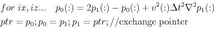
where
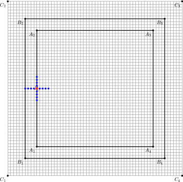
As you see, RTM begs for an accurate reconstruction before applying the imaging condition using the backward propagated wavefield. The velocity model is typically extended with sponge absorbing boundary condition (ABC) (Cerjan et al., 1985) or PML and its variants (Komatitsch and Martin, 2007) to a larger size. In Figure 1, the original model size
![]() is extended to
is extended to
![]() . In between is the artificial boundary (
. In between is the artificial boundary (
![]() ).
Actually, the wavefield we intend to reconstruct is not the part in extended artificial boundary
).
Actually, the wavefield we intend to reconstruct is not the part in extended artificial boundary
![]() but the part in the original model zone
but the part in the original model zone
![]() . We can reduce the boundary load further (from whole
. We can reduce the boundary load further (from whole
![]() to part of it
to part of it
![]() ) depending on the required grids in finite difference scheme, as long as we can maintain the correctness of wavefield in
) depending on the required grids in finite difference scheme, as long as we can maintain the correctness of wavefield in
![]() . We do not care about the correctness of the wavefield neither in
. We do not care about the correctness of the wavefield neither in
![]() nor in the effective zone
nor in the effective zone
![]() (i.e. the wavefield in
(i.e. the wavefield in
![]() ). Furthermore, we only need to compute the imaging condition in the zone
). Furthermore, we only need to compute the imaging condition in the zone
![]() , no concern with the part in
, no concern with the part in
![]() .
.
|
|---|
|
fig1
Figure 1. Extend the model size with artificial boundary. |
|
|
|
|
|
|
RTM using effective boundary saving: A staggered grid GPU implementation |