|
|
|
|
RTM using effective boundary saving: A staggered grid GPU implementation |
To make sure that the proposed effective boundary saving strategy does not introduce any kind of error/artifacts for the source wavefield, the first example is designed using a constant velocity model: velocity=2000 m/s, ![]() ,
,
![]() . The source position is set at the center of the model. The modeling process is performed
. The source position is set at the center of the model. The modeling process is performed ![]() time samples. We record the modeled wavefield snap at
time samples. We record the modeled wavefield snap at ![]() and
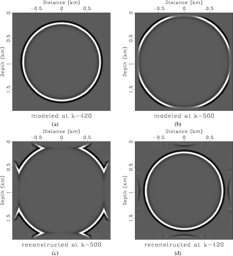
and ![]() , as shown in the top panels of Figure 6. The backward propagation starts from
, as shown in the top panels of Figure 6. The backward propagation starts from ![]() and ends up with
and ends up with ![]() . In the backward steps, the reconstructed wavefield at
. In the backward steps, the reconstructed wavefield at ![]() and
and ![]() are also recorded, shown in the bottom panels of Figure 6. We also plot the wavefield in the boundary zone in both two panels. Note that the correctness of the wavefield in the original model zone is guaranteed while the wavefield in the boundary zone does not need to be correct.
are also recorded, shown in the bottom panels of Figure 6. We also plot the wavefield in the boundary zone in both two panels. Note that the correctness of the wavefield in the original model zone is guaranteed while the wavefield in the boundary zone does not need to be correct.
|
|---|
|
fig6
Figure 6. The wavefield snaps with a constant velocity model: velocity=2000 m/s, |
|
|
|
|
|
|
RTM using effective boundary saving: A staggered grid GPU implementation |