A graphics processing unit implementation of time-domain full-waveform inversion

Acknowledgments

The work of the first author is supported by China Scholarship Council during his visit to Bureau of Economic Geology, The University of Texas at Austin. This work is sponsored by National Science Foundation of China (No. 41390454). Thanks go to IFP for the Marmousi model. We wish to thank Sergey Fomel for valuable help to incorporate the codes into Madagascar software package (Fomel et al., 2013) (http://www.ahay.org), which makes all the numerical examples reproducible. The paper is substantially improved according to the suggestions of Joe Dellinger, Robin Weiss and two other reviewers.

Appendix A

Misfit function minimization

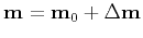
Here, we mainly follow the delineations of FWI by Pratt et al. (1998) and Virieux and Operto (2009).The minimum of the misfit function $E(\textbf{m})$ is sought in the vicinity of the starting model $\textbf{m}_0$ . The FWI is essentially a local optimization. In the framework of the Born approximation, we assume that the updated model $\textbf{m}$ of dimension $M$ can be written as the sum of the starting model $\textbf{m}_0$ plus a perturbation model $\Delta \textbf{m}$ : $\textbf{m}=\textbf{m}_0+\Delta \textbf{m}$ . In the following, we assume that $\textbf{m}$ is real valued.

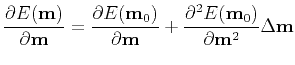
A second-order Taylor-Lagrange development of the misfit function in the vicinity of $\textbf{m}_0$ gives the expression

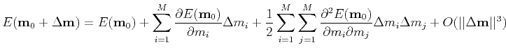$$E(\textbf{m}_0+\Delta \textbf{m})=E(\textbf{m}_0) +\sum_{i=1}^M\f... ..._i \partial m_j}\Delta m_i \Delta m_j+O(\vert\vert\Delta\textbf{m}\vert\vert^3)$$ (17)

Taking the derivative with respect to the model parameter $m_i$ results in

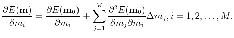$$\frac{\partial E(\textbf{m})}{\partial m_i}=\frac{\partial E(\tex... ...artial^2 E(\textbf{m}_0)}{\partial m_j \partial m_i}\Delta m_j, i=1,2,\ldots,M.$$ (18)

Equation (A-2) can be abbreviated as

$$\frac{\partial E(\textbf{m})}{\partial \textbf{m}}=\frac{\partial... ...bf{m}}+\frac{\partial^2 E(\textbf{m}_0)}{\partial\textbf{m}^2}\Delta \textbf{m}$$ (19)

Thus,

$$\Delta \textbf{m}=-\left(\frac{\partial^2 E(\textbf{m}_0)}{\parti... ...ial E(\textbf{m}_0)}{\partial \textbf{m}}=-\textbf{H}^{-1}\nabla E_{\textbf{m}}$$ (20)

where

$$\nabla E_{\textbf{m}}=\frac{\partial E(\textbf{m}_0)}{\partial \t... ...}{\partial m_2}, \ldots, \frac{\partial E(\textbf{m}_0)}{\partial m_M}\right]^T$$ (21)

and

$$\textbf{H}=\frac{\partial^2 E(\textbf{m}_0)}{\partial\textbf{m}^2} =\left(\frac{\partial^2 E(\textbf{m}_0)}{\partial m_i\partial m_j}\right)$$ (22)

$\nabla E_{\textbf{m}}$ and $\textbf{H}$ are the gradient vector and the Hessian matrix, respectively.

$$\nabla E_{\textbf{m}}=\nabla E(\textbf{m})=\frac{\partial E(\text... ...textbf{p}\right] =\mathtt{Re}\left[\textbf{J}^{\dagger}\Delta \textbf{p}\right]$$ (23)

where $\mathtt{Re}$ takes the real part, and $\textbf{J}=\frac{\partial \textbf{f}(\textbf{m})}{\partial \textbf{m}}$ is the Jacobian matrix, i.e., the sensitivity or the Fréchet derivative matrix.

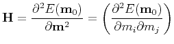
In matrix form

$$\textbf{H}=\frac{\partial^2 E(\textbf{m})}{\partial \textbf{m}^2}... ...(\Delta \textbf{p}^*, \Delta \textbf{p}^*, \ldots, \Delta \textbf{p}^*)\right].$$ (24)

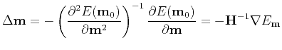
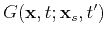
In the Gauss-Newton method, this second-order term is neglected for nonlinear inverse problems. In the following, the remaining term in the Hessian, i.e., $\textbf{H}_a=\mathtt{Re}[\textbf{J}^{\dagger}\textbf{J}]$ , is referred to as the approximate Hessian. It is the auto-correlation of the derivative wavefield. Equation (A-4) becomes

$$\Delta \textbf{m} =-\textbf{H}^{-1}\nabla E_{\textbf{m}} =-\textbf{H}_a^{-1}\mathtt{Re}[\textbf{J}^{\dagger}\Delta \textbf{p}].$$ (25)

To guarantee the stability of the algorithm (avoiding the singularity), we may use 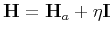$\textbf{H}=\textbf{H}_a+\eta \textbf{I}$ , leading to

$$\Delta \textbf{m} =-\textbf{H}^{-1}\nabla E_{\textbf{m}} =-(\text... ... \textbf{I})^{-1}\mathtt{Re}\left[\textbf{J}^{\dagger}\Delta \textbf{p}\right].$$ (26)

Alternatively, the inverse of the Hessian in equation (A-4) can be replaced by $\textbf{H}=\textbf{H}_a\approx\mu \textbf{I}$ , leading to the gradient or steepest-descent method:

$$\Delta \textbf{m} =-\mu^{-1}\nabla E_{\textbf{m}} =-\alpha\nabla ... ...xtbf{m}} =-\alpha\mathtt{Re}\left[\textbf{J}^{\dagger}\Delta \textbf{p}\right].$$ (27)

where $\alpha=\mu^{-1}$ .

Appendix B

Fréchet derivative

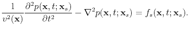
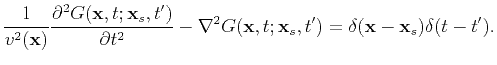
Recall that the basic acoustic wave equation reads

$$\frac{1}{v^2(\textbf{x})}\frac{\partial^2 p(\textbf{x},t;\textbf{... ...tial t^2}-\nabla^2 p(\textbf{x},t;\textbf{x}_s)=f_s(\textbf{x},t;\textbf{x}_s).$$

The Green's function $G(\textbf{x},t;\textbf{x}_s,t')$ is defined by

$$\frac{1}{v^2(\textbf{x})}\frac{\partial^2 G(\textbf{x},t;\textbf{... ... G(\textbf{x},t; \textbf{x}_s,t') =\delta(\textbf{x}-\textbf{x}_s)\delta(t-t').$$ (28)

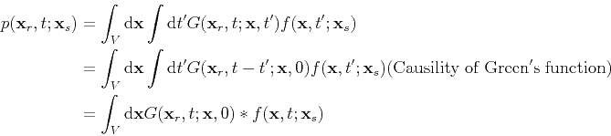
Thus the integral representation of the solution can be given by (Tarantola, 1984)

$$\begin{split}p(\textbf{x}_r,t; \textbf{x}_s)&=\int_V \mathrm{... ...f{x}_r,t;\textbf{x},0)*f(\textbf{x},t;\textbf{x}_s) \end{split}$$ (29)

where $*$ denotes the convolution operator.

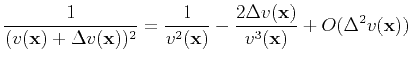
A perturbation $v(\textbf{x})\rightarrow v(\textbf{x})+\Delta v(\textbf{x})$ will produce a field $p(\textbf{x},t;\textbf{x}_s)+\Delta p(\textbf{x},t;\textbf{x}_s)$ defined by

$$\frac{1}{(v(\textbf{x})+\Delta v(\textbf{x}))^2}\frac{\partial^2 ... ...xtbf{x}_s)+\Delta p(\textbf{x},t;\textbf{x}_s)] =f_s(\textbf{x},t;\textbf{x}_s)$$ (30)

Note that

$$\frac{1}{(v(\textbf{x})+\Delta v(\textbf{x}))^2} =\frac{1}{v^2(\textbf{x})}-\frac{2\Delta v(\textbf{x})}{v^3(\textbf{x})}+O(\Delta^2 v(\textbf{x}))$$ (31)

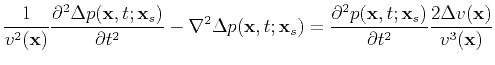
Equation (B-3) subtracts equation (1), yielding

$$\frac{1}{v^2(\textbf{x})}\frac{\partial^2 \Delta p(\textbf{x},t;\... ...x},t;\textbf{x}_s)]}{\partial t^2}\frac{2\Delta v(\textbf{x})}{v^3(\textbf{x})}$$ (32)

Using the Born approximation, equation (B-5) becomes

$$\frac{1}{v^2(\textbf{x})}\frac{\partial^2 \Delta p(\textbf{x},t;\... ...{x},t;\textbf{x}_s)}{\partial t^2}\frac{2\Delta v(\textbf{x})}{v^3(\textbf{x})}$$ (33)

Again, based on integral representation, we obtain

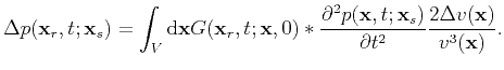$$\Delta p(\textbf{x}_r,t; \textbf{x}_s)=\int_V \mathrm{d}\textbf{x... ...x},t;\textbf{x}_s)}{\partial t^2}\frac{2\Delta v(\textbf{x})}{v^3(\textbf{x})}.$$ (34)

Appendix C

Gradient computation

In terms of equation (2),

$$\begin{split}\frac{\partial E(\textbf{m})}{\partial m_i} &=\f... ...^{\dagger}\Delta \textbf{p}\right], i=1,2,\ldots,M. \end{split}$$ (35)

According to the previous section, it follows that

$$\frac{\partial p_{cal}}{\partial v_i(\textbf{x})} =\int_V \mathrm... ...partial^2 p(\textbf{x},t;\textbf{x}_s)}{\partial t^2}\frac{2}{v^3(\textbf{x})}.$$ (36)

The convolution guarantees

$$\int \mathrm{d}t [g(t)*f(t)]h(t)=\int \mathrm{d}t f(t)[g(-t)*h(t)].$$ (37)

Then, equation (C-1) becomes

$$\begin{split}\frac{\partial E(\textbf{m})}{\partial m_i} &=\s... ...ght)^*p_{res}(\textbf{x}_r,t;\textbf{x}_s)\right]\\ \end{split}$$ (38)

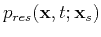where $p_{res}(\textbf{x},t;\textbf{x}_s)$ is a time-reversal wavefield produced using the residual $\Delta p(\textbf{x}_r,t;\textbf{x}_s)$ as the source. As follows from reciprocity theorem,

$$p_{res}(\textbf{x},t;\textbf{x}_s) =\int_V \mathrm{d}\textbf{x} G... ...textbf{x} G(\textbf{x},0;\textbf{x}_r,t)*\Delta p(\textbf{x}_r,t;\textbf{x}_s).$$ (39)

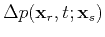
satisfying

$$\frac{1}{v^2(\textbf{x})}\frac{\partial^2 p_{res}(\textbf{x},t;\t... ...bla^2 p_{res}(\textbf{x},t;\textbf{x}_s)=\Delta p(\textbf{x}_r,t;\textbf{x}_s).$$ (40)

It is noteworthy that an input $f$ and the system impulse response function $g$ are exchangeable in convolution. That is to say, we can use the system impulse response function $g$ as the input, the input $f$ as the impulse response function, leading to the same output. In the seismic modeling and acquisition process, the same seismogram can be obtained when we shoot at the receiver position $\textbf{x}_r$ when recording the seismic data at position $\textbf{x}$ .

A graphics processing unit implementation of time-domain full-waveform inversion