Solving 3D Anisotropic Elastic Wave Equations on Parallel GPU Devices

Numerical approach

Any numerical implementation of equations 1-3 requires specifying both a computational mesh and a numerical discritization scheme. We define a $N_x \times N_y \times N_z$ computational grid and use $N_t$ time steps such that a grid point in space and time can be represented by quadruplet $[x,y,z\vert t]=[p \Delta x, q \Delta y, r\Delta z\vert n\Delta t]$ , where the integer counters have the ranges $p=1,N_x$ , $q=1,N_y$ , $r=1,N_z$ and $n=1,N_t$ . Continuous wavefield displacements at a given location are represented on the discritized grid as

$$u_i\left\vert _{x,y,z\vert t} \right. \approx u_i^{p,r,q\vert n}.$$ (4)

We approximate the first derivative $\partial_j$ by a compact centered difference operator $D_x[\cdot]$ of 8$^{th}$ -order accuracy (Trefethen, 1996)

$$\partial_x u_j \approx D_x [ u_j^{p,q,r\vert n}] = \frac{1}{\Delt... ...^4 W_\alpha \left( u^{p+\alpha,q,r\vert n}_j-u^{p-\alpha,q,r\vert n}_j \right),$$ (5)

where $W_\alpha$ are polynomial weights given by ${\bf W}=\left[\frac{+4}{5}\, \frac{-1}{5} \, \frac{+4}{105} \, \frac{-1}{280} \right]$ . Spatial difference operators $D_y[\cdot]$ and $D_z[\cdot]$ are specified similarly for the $y-$ and $z-$ directional derivatives, and all three are used for derivatives of the constitutive relationship in equation 3 (i.e., $\partial_j c_{ijkl}$ ). We use a standard second-order accuracy approximation for the second time derivative in equation 3

$$\partial^2_{tt} u_j \approx D_{tt} u_j^{p,q,r\vert n} = \frac{1}{... ... \left[ u_j^{p,q,r\vert n+1}-2 u_j^{p,q,r\vert n}+u_j^{p,q,r\vert n-1} \right].$$ (6)

Inserting the above difference operators into equations 1-3 and rearranging terms leads to a FD scheme for calculating the unknown wavefield solution at the forward time step, $u_j^{p,q,r\vert n+1}$ , given wavefield values at the current and previous time steps, $u_j^{p,q,r\vert n}$ and $u_j^{p,q,r\vert n-1}$ , and stencil points neighboring $u_j^{p,q,r\vert n}$ in the $x$ -, $y$ - and $z$ -directions. Figure 1 depicts the FD stencil constructed from the points about $u_j^{p,q,r\vert n}$ at the current time step.

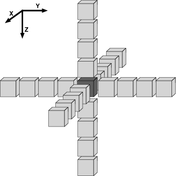
starOfCubes
Figure 1. The 25 data points required to approximate a first derivative at the center shaded point using a FD stencil of 8$^{th}$ -order accuracy.

These difference operators allow us to specify a time-stepping scheme to calculate wavefield displacements in 3D elastic anisotropic media throughout the model domain. However, additional work is required to treat both the free-surface boundary and to minimize the energy in non-physical exterior boundary reflections. Implementing free-surface boundary conditions is fairly straightforward on a uniform grid because a (topography-free) free surface can be placed directly on the boundary which, assuming the free-surface normal vector points in the $z$ -direction, allows us to set $\sigma_{i3}=0$ where $i=1,2,3$ . We treat the other boundaries using a cascade of two operators comprised of absorbing boundary conditions (ABCs) derived from a one-way wave equation (Clayton and Enquist, 1977) and an exponential-damping sponge layer (Cerjan et al., 1985) of at least 48 grid points.

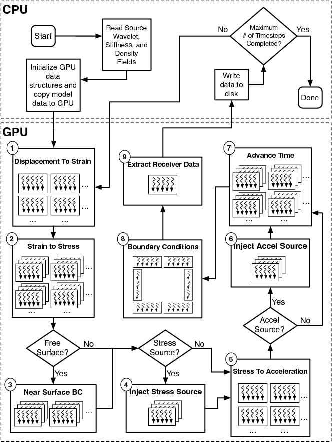
Figure 2 presents the nine procedural steps in the 3D FDTD algorithm required for calculating each forward time-step: 1) Compute strains $\epsilon_{kl}$ from wavefield displacements according to equation 1; 2) Calculate stresses $\sigma_{ij}$ from constitutive relationship $c_{ijkl}$ and $\epsilon_{kl}$ according to equation 2; 3) Enforce the free-surface boundary condition (if required); 4) Inject a stress source (if not an acceleration source); 5) Compute acceleration from stress tensor (i.e., $RHS = \partial_j \sigma_{ij}$ ); 6) Inject an acceleration source (if not a stress source; $RHS \stackrel{+}{=} F_{j}$ ); 7) Compute the forward time step from current and previous wavefield values; 8) Apply boundary conditions through cascade of ABC and sponge operators; and 9) Output data/wavefield as required. The next section details our GPU implementation of these steps.

flow
Figure 2. Control flow for FDTD algorithm implemented on a single GPU, including the division of tasks between the CPU host and GPU device.

Solving 3D Anisotropic Elastic Wave Equations on Parallel GPU Devices