|
|
|
|
A variational approach for picking optimal surfaces from semblance-like panels |
The semblance-like volume for horizon likelihood employed here is less advanced than some of those appearing in the literature. In our approach, which is detailed in Appendix ![]() , a trace representative of a seismic horizon is selected, cosine tapering is applied to its edges, and it is padded with zeros. To measure how well that ideal waveform matches with other traces throughout the seismic image volume, the crosscorrelation is calculated throughout the volume over shift
, a trace representative of a seismic horizon is selected, cosine tapering is applied to its edges, and it is padded with zeros. To measure how well that ideal waveform matches with other traces throughout the seismic image volume, the crosscorrelation is calculated throughout the volume over shift ![]() . The minimum crosscorrelation value is subtracted so the output semblance-like volume is non-negative. Automatic picking may be performed on that volume to determine the shifts defining the horizon. Those shifts may be converted back to time in the image domain by adding a reference time for the reference horizon trace, taken here to be the trace's midpoint.
. The minimum crosscorrelation value is subtracted so the output semblance-like volume is non-negative. Automatic picking may be performed on that volume to determine the shifts defining the horizon. Those shifts may be converted back to time in the image domain by adding a reference time for the reference horizon trace, taken here to be the trace's midpoint.
|
|---|
|
hcube,hcube-w
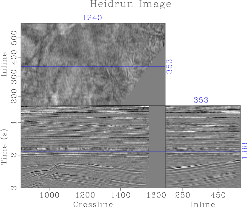
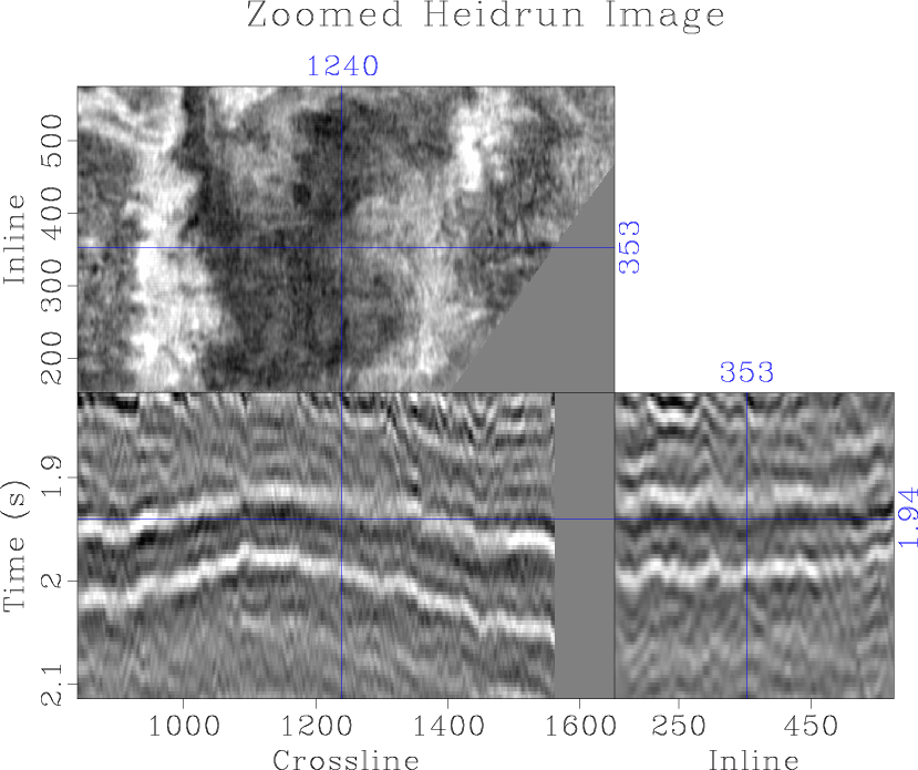
Figure 15. (a) Seismic image from the Heidrun Field; (b) zoomed portion of that image centered on the horizon that will be automatically picked. |
|
|
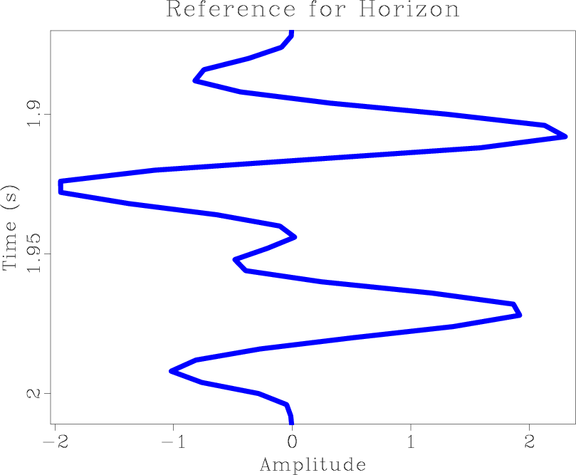
Figure 15a contains a seismic image from the Heidrun Field off the coast of Norway, and Figure 15b contains a zoomed portion of that image. We will focus on automatically picking the horizon defined by the ``double white peak'' in Figure 15b. A waveform representing an ideal version of that horizon is selected, and that horizon reference trace is plotted in Figure 16.
|
|---|
|
heidrun-reference
Figure 16. Reference trace for horizon that will be picked from Figure 15b. |
|
|
|
|---|
|
heidrun-alpha-scalebar
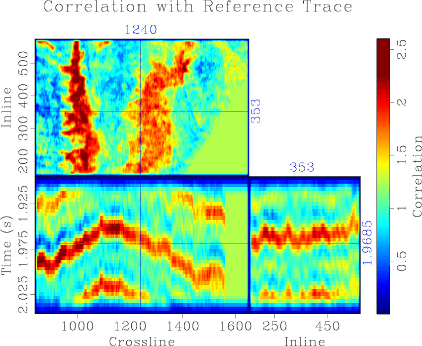
Figure 17. Cross correlation between reference trace and seismic image. |
|
|
Crosscorrelation values between the horizon reference trace and the seismic image are computed over a variety of shifts according to Equations B-1 and B-2. The shift coordinate ![]() is transformed to image time
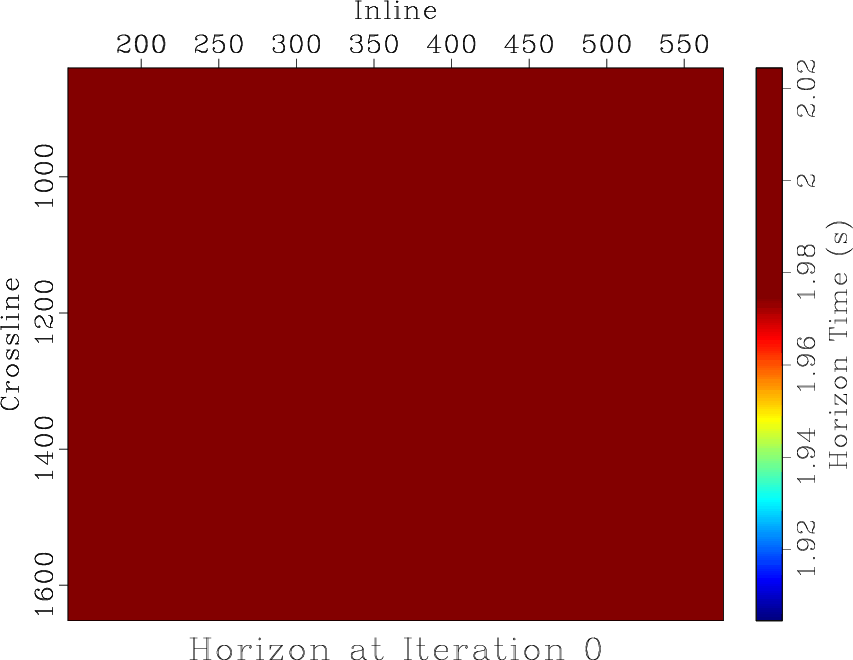
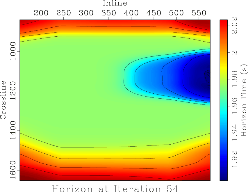
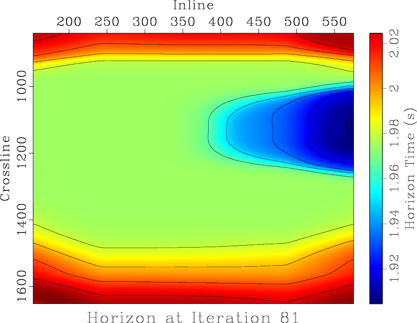
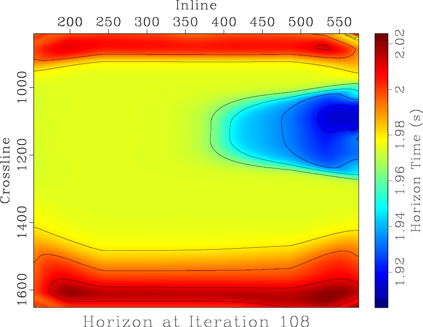
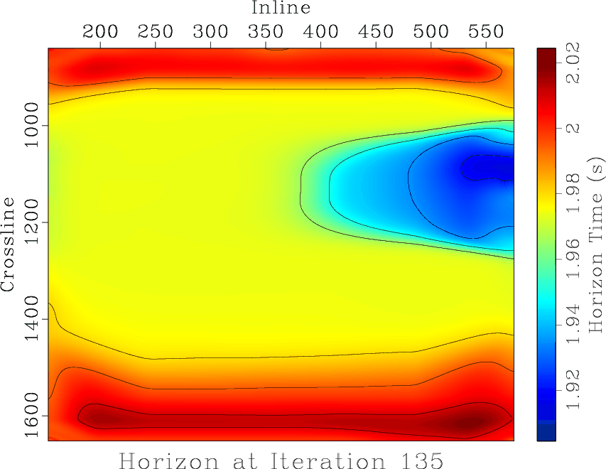
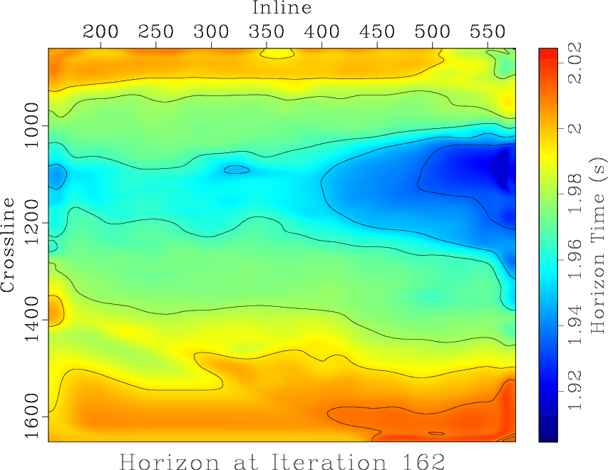
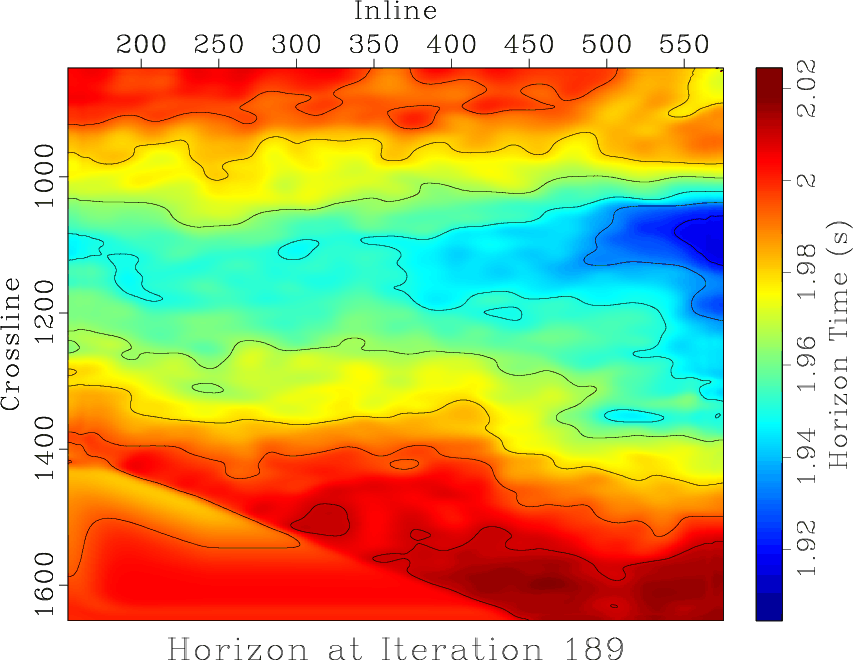
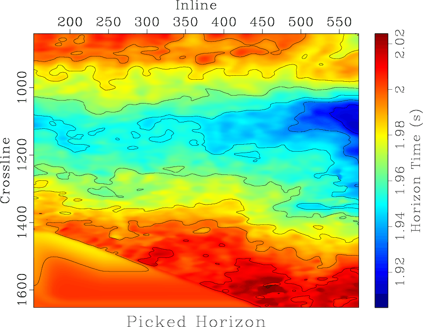
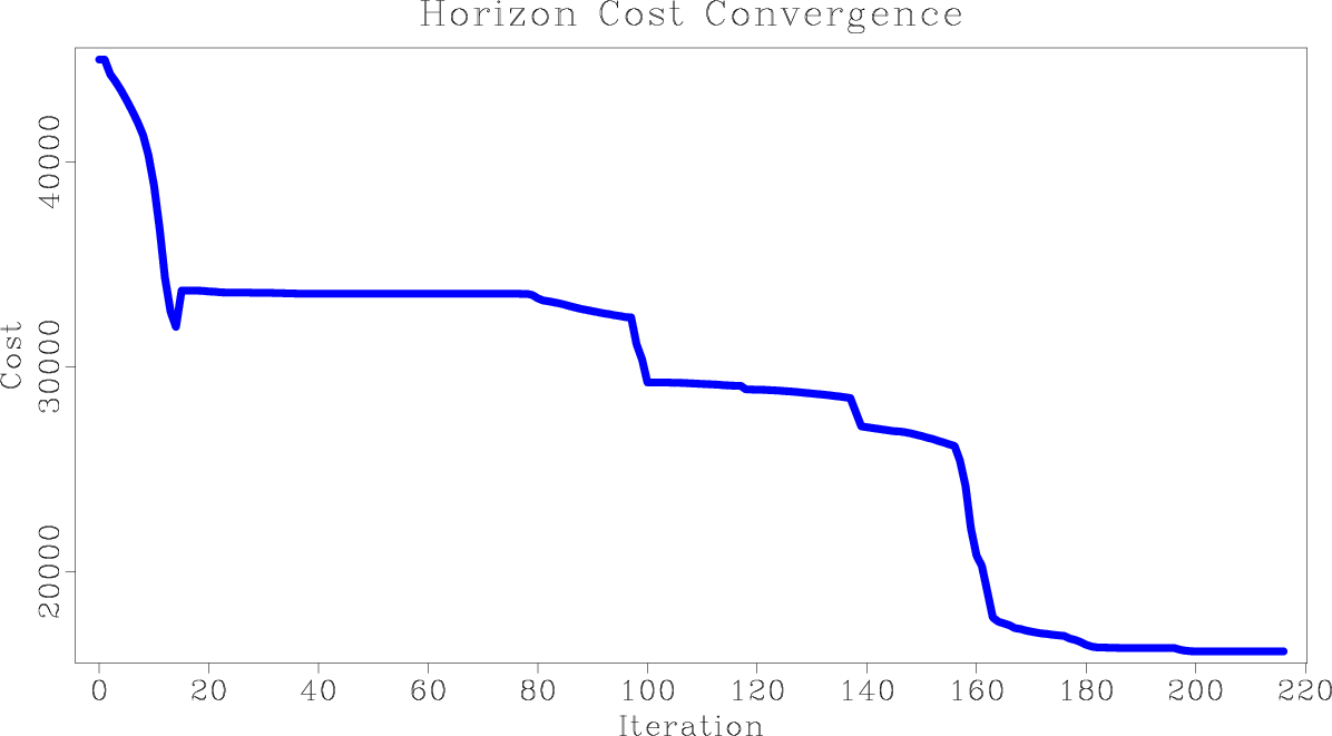
is transformed to image time ![]() to be representative of horizon location and displayed in Figure 17. Continuation picking is applied to the crosscorrelation volume using a flat starting model of 1.9745 s using 12 continuation levels. The evolution of the picked horizon every ten iterations, beginning with the starting model, is shown in Figures 18a through 18i. The final picked horizon is shown with constant horizon time contours in Figure 19. The cost convergence is calculated for each model update using the semblance-like volume in Figure 17 and displayed in Figure 20.
to be representative of horizon location and displayed in Figure 17. Continuation picking is applied to the crosscorrelation volume using a flat starting model of 1.9745 s using 12 continuation levels. The evolution of the picked horizon every ten iterations, beginning with the starting model, is shown in Figures 18a through 18i. The final picked horizon is shown with constant horizon time contours in Figure 19. The cost convergence is calculated for each model update using the semblance-like volume in Figure 17 and displayed in Figure 20.


|
|---|
|
heidrun-starting-updates-itr-0-contour,heidrun-starting-updates-itr-1-contour,heidrun-starting-updates-itr-2-contour,heidrun-starting-updates-itr-3-contour,heidrun-starting-updates-itr-4-contour,heidrun-starting-updates-itr-5-contour,heidrun-starting-updates-itr-6-contour,heidrun-starting-updates-itr-7-contour,heidrun-starting-updates-itr-8-contour
Figure 18. Evolution of continuation picking horizon overlaid by constant horizon time contours. |
|
|
|
|---|
|
heidrun-horiz-out-11-contour
Figure 19. Final picked horizon with constant horizon time contours. |
|
|
|
|---|
|
heidrun-starting-updates-costs
Figure 20. Cost convergence for continuation horizon picking using the semblance-like volume shown in Figure 17. |
|
|
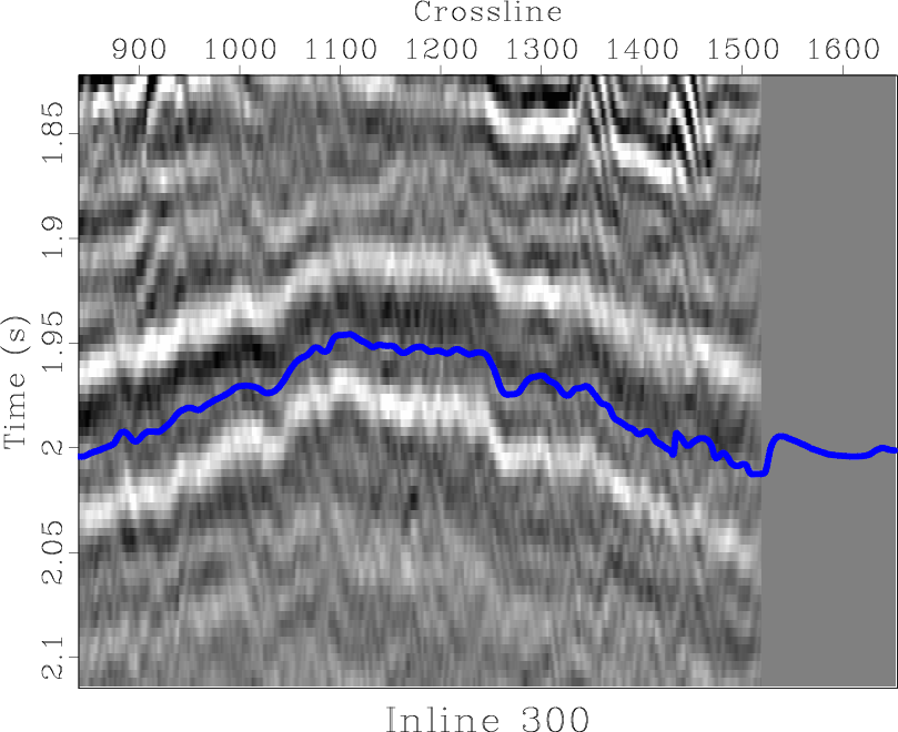
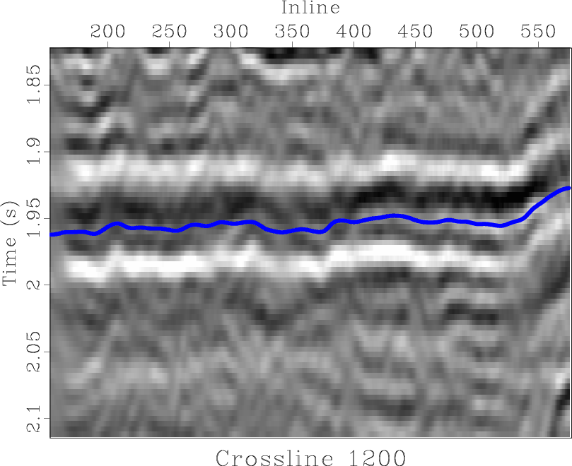
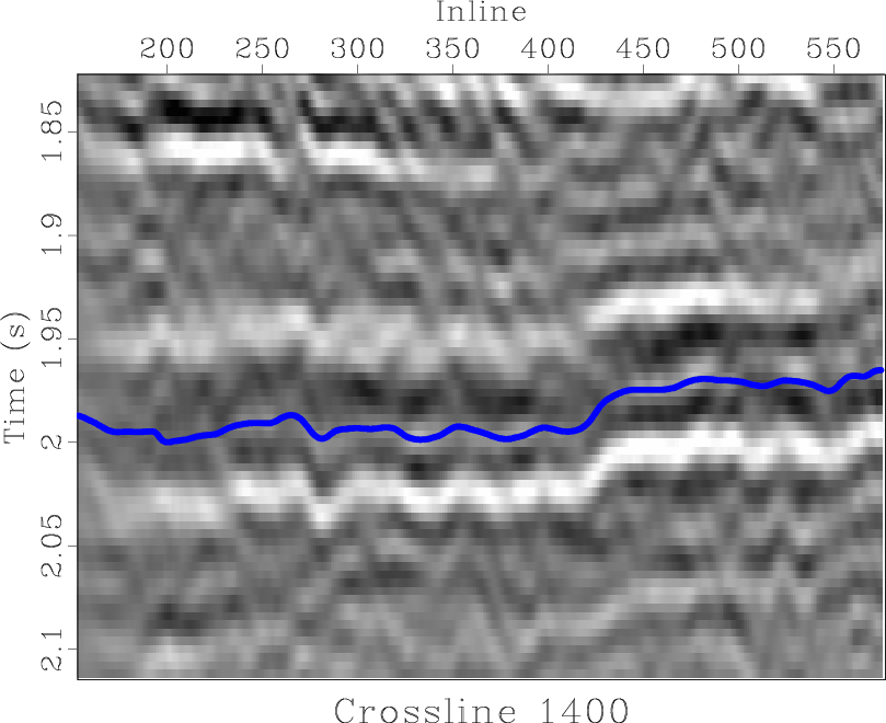
To illustrate the picked horizon in the seismic volume, we generate a series of overlay images. Note that the position of the horizon is taken to be at the halfway point of the reference trace in Figure 16, and thus we would expect it to approximately track the trough between the double white peaks in the image. Constant-inline slices are shown for inline 100 in Figure 21a and inline 300 in Figure 21b. Constant-crossline slices are similarly generated and shown for crossline 1200 in Figure 21c and crossline 1400 in Figure 21d.

|
|---|
|
hcube-wind-il-overlay-0,hcube-wind-il-overlay-2,hcube-wind-xl-overlay-1,hcube-wind-xl-overlay-3
Figure 21. Picked horizon from Figure 19 overlaid on Heidrun seismic image from Figure 15b for: (a) Inline 100; (b) Inline 300; (c) Crossline 1200; (d) Crossline 1400. |
|
|
The variational picking method outlined here appears to successfully pick the desired horizon from a poorly informed, flat starting model. Examining the picked horizon image overlays (Figures 21a through 21d) the horizon successfully tracks the trough between the two bright, white peaks, even when that position changes relatively rapidly, as is the case near crossline 1050 in Figure 21a, or when the character of the horizon wavelet changes somewhat, as is the case near inline 560 in Figure 21d. The display of the picked horizon in Figure 19 shows how the method is able to identify a plunging anticline structure in the horizon. The horizon-quality-of-fit volume defined by Equation B-2 is primitive, and may not be well-suited for the automatic interpretation of other horizons which are faulted or where there are significant changes in the wavelet. However, when applied to the horizon in this study, and used in conjunction with the continuation-variational picking method, it is able to produce a representation of the horizon from the single seed wavelet shown in Figure 16. When used with more sophisticated measures of horizon location probability, the variational approach outlined here could help produce high-quality automatic interpretations of subsurface features with minimal human intervention.
|
|
|
|
A variational approach for picking optimal surfaces from semblance-like panels |