|
|
|
|
A robust approach to time-to-depth conversion and interval velocity estimation from time migration in the presence of lateral velocity variations |
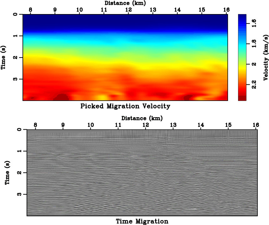
The field data shown in Figure 17 is from a section of Gulf of Mexico dataset (Claerbout, 1996). We
estimate ![]() using the method of velocity continuation (Fomel, 2003) and convert it to
using the method of velocity continuation (Fomel, 2003) and convert it to ![]() . Similar to
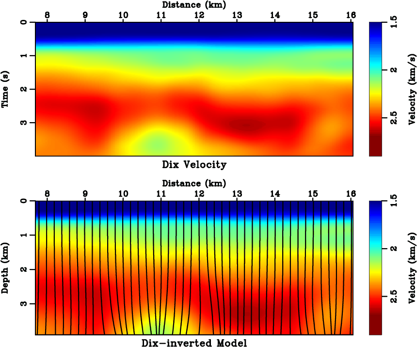
the spiral model, no domain extension is needed. In Figure 18, the Dix-inverted prior model highly
resembles the Dix velocity, because the Dix formula only scales the vertical axis from time to depth regardless
of horizontal
. Similar to
the spiral model, no domain extension is needed. In Figure 18, the Dix-inverted prior model highly
resembles the Dix velocity, because the Dix formula only scales the vertical axis from time to depth regardless
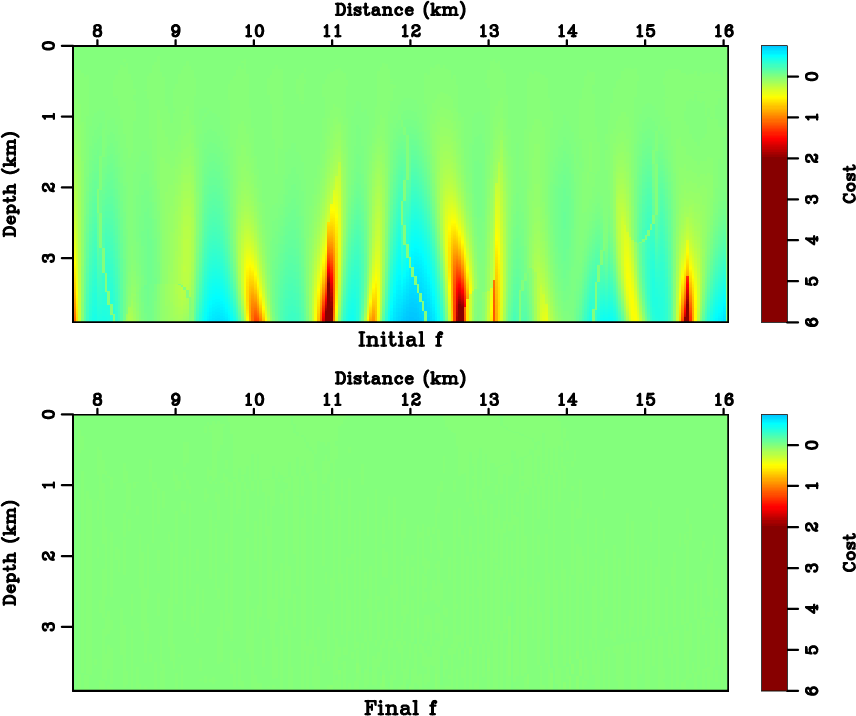
of horizontal ![]() variations. Figure 19 compares the cost before and after five linearization
updates, with a
variations. Figure 19 compares the cost before and after five linearization
updates, with a ![]() m
m ![]()
![]() m triangular smoother. In Figure 20, the
m triangular smoother. In Figure 20, the
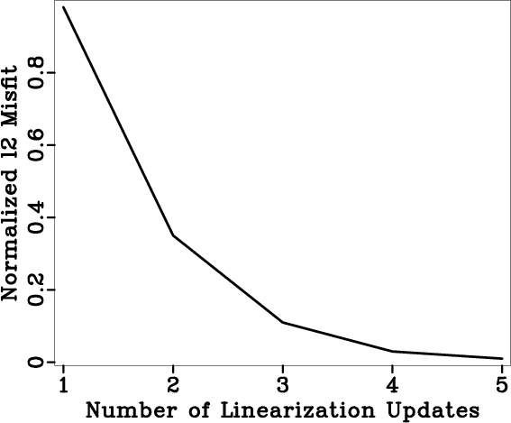
![]() norm of the cost,
norm of the cost, ![]() , has a rapid decrease to relative
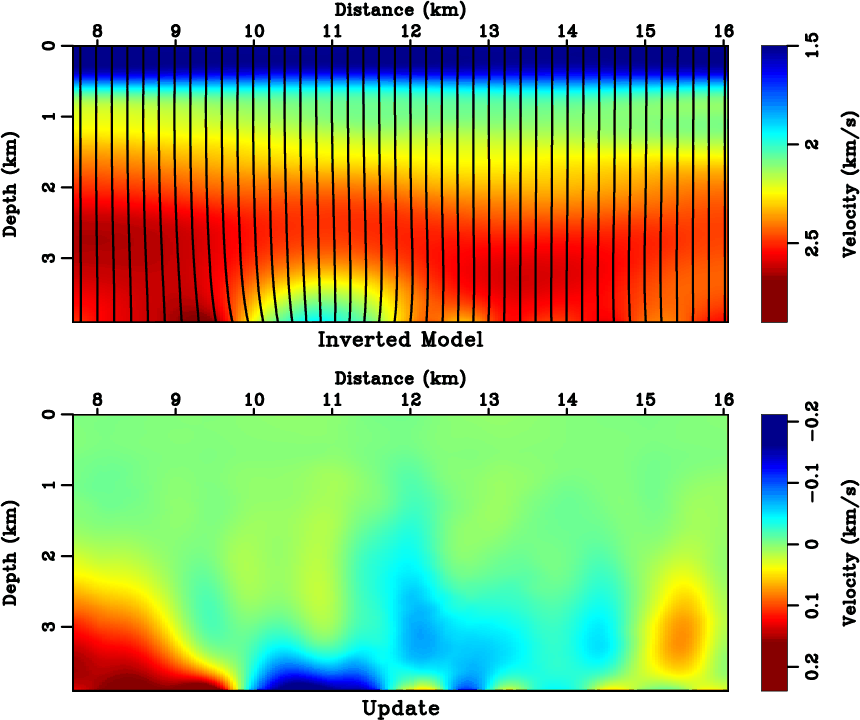
, has a rapid decrease to relative ![]() %. Figure 21 illustrates the
inverted model and interval velocity update.
%. Figure 21 illustrates the
inverted model and interval velocity update.
|
|---|
|
vdix
Figure 17. (Top) the estimated time-migration velocity of a section of Gulf of Mexico dataset and (bottom) the corresponding time-migrated image. |
|
|
|
|---|
|
init
Figure 18. (Top) the Dix velocity converted from |
|
|
|
|---|
|
inv
Figure 19. The cost of (top) prior model ( |
|
|
|
hist
Figure 20. Convergence history of the proposed optimization-based time-to-depth conversion. |
|
|---|---|
|
|
|
|---|
|
dinv
Figure 21. (Top) the inverted model, overlaid with image rays, and (bottom) its difference from the prior model in Figure 18. |
|
|
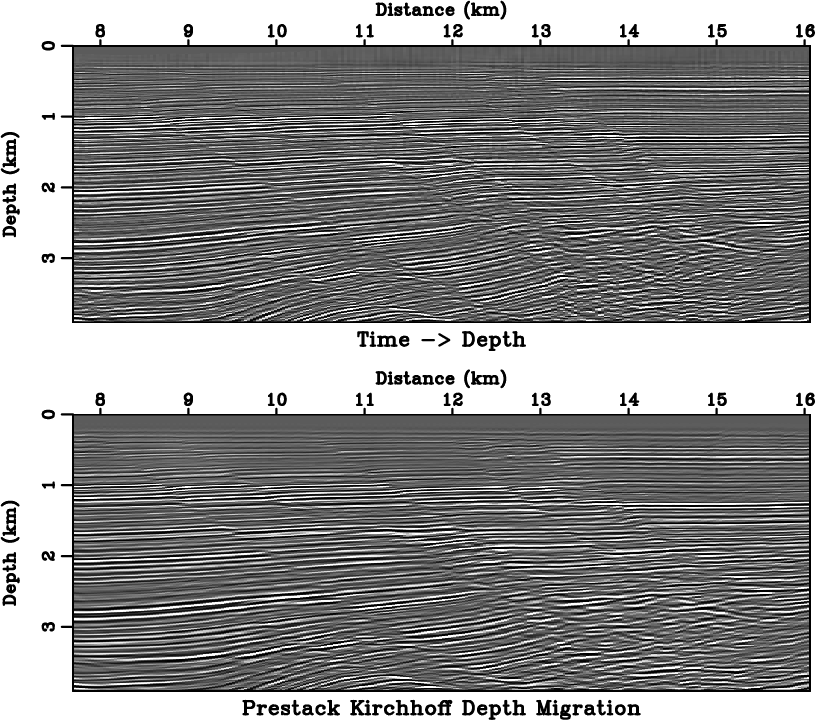
Next, we map the time-migrated image to depth using ![]() and
and ![]() generated during inversion. Spline
interpolation (Press et al., 2007) is used during the coordinate mapping. We also migrate the
prestack data by Kirchhoff depth migration (Li and Fomel, 2013) (PSDM). Figure 22 compares the
time-mapped image and PSDM image of the inverted model. A good agreement between these two images justifies that
time-to-depth conversion has effectively unravelled the distorted time coordinate. Figure 23 compares
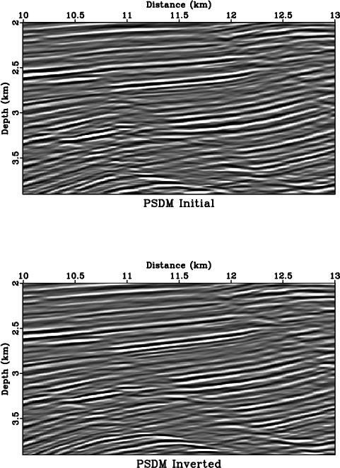
PSDM images of the prior and inverted models. The velocity update in Figure 21 results in not only
changes in structural dips (for example at
generated during inversion. Spline
interpolation (Press et al., 2007) is used during the coordinate mapping. We also migrate the
prestack data by Kirchhoff depth migration (Li and Fomel, 2013) (PSDM). Figure 22 compares the
time-mapped image and PSDM image of the inverted model. A good agreement between these two images justifies that
time-to-depth conversion has effectively unravelled the distorted time coordinate. Figure 23 compares
PSDM images of the prior and inverted models. The velocity update in Figure 21 results in not only
changes in structural dips (for example at ![]() km) but also improved reflector continuity (for example at
km) but also improved reflector continuity (for example at
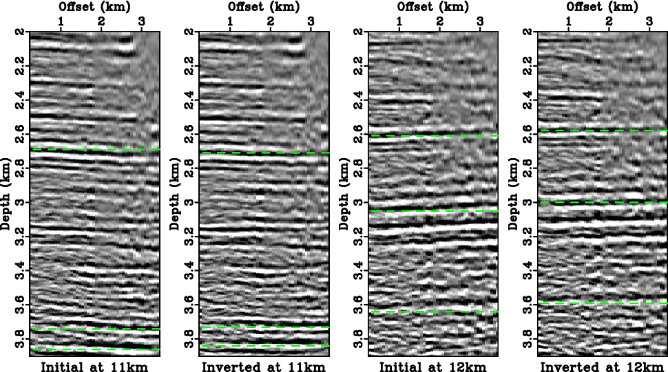
![]() km). Moreover, the Kirchhoff migration outputs surface offset common-image
gathers. We choose two midpoint locations,
km). Moreover, the Kirchhoff migration outputs surface offset common-image
gathers. We choose two midpoint locations, ![]() km and
km and ![]() km,
and show their common-image gathers in Figure 24. In deeper sections, flat dashed lines are
overlaid as references for the
flatness of gathers. The two common-image gathers of prior model appear curved in opposite directions. After
time-to-depth conversion, both gathers get flattened across the whole offset range,
verifying a correct velocity update.
km,
and show their common-image gathers in Figure 24. In deeper sections, flat dashed lines are
overlaid as references for the
flatness of gathers. The two common-image gathers of prior model appear curved in opposite directions. After
time-to-depth conversion, both gathers get flattened across the whole offset range,
verifying a correct velocity update.
|
|---|
|
dmig
Figure 22. (Top) the time-migrated image in Figure 17 is mapped to depth using products of the time-to-depth conversion. (Bottom) PSDM image using inverted model in Figure 21. |
|
|
|
|---|
|
ddmig0
Figure 23. PSDM images of (top) the prior model and (bottom) the inverted model. Both images are plotted for the same central deep part. |
|
|
|
|---|
|
cig0
Figure 24. The surface offset common-image gathers of prior and inverted models. |
|
|
|
|
|
|
A robust approach to time-to-depth conversion and interval velocity estimation from time migration in the presence of lateral velocity variations |