|
 |
 |
 | Fast time-to-depth conversion and interval velocity estimation in the case of weak lateral variations |  |
![[pdf]](icons/pdf.png) |
Next: Examples
Up: Theory
Previous: Theory
Instead of attempting to solve equations 5-7 directly, we assume that the lateral variations are mild and the parameters can be approximated with respect to the laterally homogeneous background up to the first-order linearization as follows:
The first terms on the right-hand side of equations 8-10 correspond to the correct values of the velocity squared  ,
,  , and
, and  for the reference laterally homogeneous background. Our objective is to seek for
  ,
,
 , and
, and
 that quantify the first-order effects from lateral heterogenity and satisfy the system of PDEs in equations 5-7. Substituting equations 8-10 into equations 5-7 and restrict our consideration only up to the first-order perturbations, we can derive
which is a considerably simpler system to solve than the original one. However, implementing the proposed system requires the knowledge of  , which is unavailable from migration velocity analysis because the Dix velocity squared
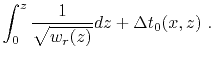
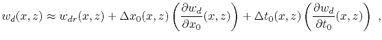
 is still expressed in the time domain. In the same spirit as before, we propose to consider instead a linearized approximation given by,
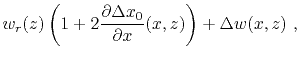
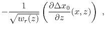
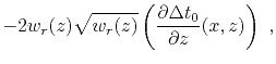
Following the similar procedure and retaining only the first-order terms, we can approximate
 and
and
 , which results in
 |
(15) |
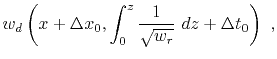
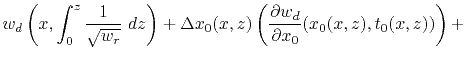
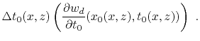
where the reference
 denotes the
converted to depth based on the laterally homogeneous background assumption, and the two derivatives are evaluated first in the original
denotes the
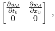
converted to depth based on the laterally homogeneous background assumption, and the two derivatives are evaluated first in the original  coordinates followed by similar conversion. Substituting equation 15 into equation 11 leads to the following first-order linear system:
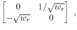
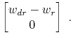
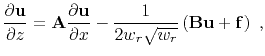 |
(16) |
where
![$ \mathbf{u} = [\Delta t_0, \Delta x_0]^T$](img65.png) ,
,
Equation 16 can be solved by stepping in the depth  direction given the following initial conditions at the surface
  :
:
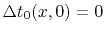 and and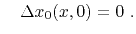 |
(20) |
In our numerical experiments, we adopt the following procedure to solve system 16:
- Provided the
from migration velocity analysis, we compute the
 and
and
 using smooth differentiation.
- Convert the velocity and both derivatives to depth based on the assumption of laterally homogeneous media to obtain
,
 , and
, and
 .
.
- Choose a reference laterally homogeneous background
 from
.
from
.
- Given the initial condition 20 on
 and other known parameters from the previous steps, we compute
 for the topmost layer using a derivative filter followed by smoothing which helps alleviate the effects from sharp contrasts and their corresponding numerical artifacts that may get carried on to the next depth step.
- We make a step in depth based on
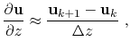 |
(21) |
where  represents the depth increment of the model, the current layer is denoted by
  and the next layer is denoted by
  .
.
- Repeat steps 4 and 5 for the next layer til the final layer.
- Compute
from the estimated
using equation 13.
|
|
|
|
| Fast time-to-depth conversion and interval velocity estimation in the case of weak lateral variations | |
|
Next: Examples
Up: Theory
Previous: Theory
2018-11-16